


 nueva página del texto (beta)
 Inglés (pdf)
 Artículo en XML
 Referencias del artículo
 Enviar artículo por email
 Citado por SciELO
  Similares en
SciELO
Similares en
SciELO 
 Permalink
1. Introduction
Since the launch of the Fermi Gamma-Ray Space Telescope, there have been counterpart
supporting monitoring programs in the entire electromagnetic spectrum, from radio
waves to X-rays (e.g. SMA, Gurwell et al.
2007; OVRO, Richards et al. 2011,
SMARTS; Bonning et al. 2012, Swift; Stroh & Falcone 2013). In particular, we
focus on the Ground-based Observational Support of the Fermi Gamma-ray Space
Telescope carried out at the University of Arizona using the 2.3m Bok (Kitt Peak)
and 1.54m Kuiper (Mt. Bigelow) telescopes operated by the Steward Observatory (SO)
(Smith et al. 2009)3. This is one of the most important monitoring
programs because it is the most complete public database of optical spectroscopy,
photometry, and polarimetry, for blazars, with the largest number of sources and
best cadence of observation4. In
this program, the spectroscopic observations are conducted with the SPOL
spectropolarimeter, which uses up to 6 configurations (apertures) corresponding to
six different slit widths (1=
Unfortunately, the instrumental broadening for each slit width is not publicly available; this has prevented us from studying the variability of the FWHM of the broad emission lines present in flat-spectrum radio quasars (FSRQ), unlike the study of flux variability previously done in various works for the Mg II λ2798 (León-Tavares et al. 2013; Chavushyan et al. 2020; Amaya-Almazán et al. 2021), Hβ (Fernandes et al. 2020), and C IV λ1549 (Amaya-Almazán et al. 2022) emission lines.
FSRQ are a subtype of blazars (Urry & Padovani 1995) characterized by their high variability across the entire electromagnetic spectrum (e.g. Aharonian et al. 2007; Amaya-Almazán et al. 2021), with variations on very different time scales, even in the same wavelength range (e.g. Fan et al. 2018; Gupta 2018). When there is a flux increase in a very short time and well above the average emission we call this phenomenon a flare. Among AGNs, flares are mostly found in blazars. There is observational evidence that the emission line flares in some blazars can be driven by non-thermal emission from the jet (e.g. León-Tavares et al. 2013; Chavushyan et al. 2020; Amaya-Almazán et al. 2021, 2022); so it is interesting to study if the emission line profile also changes during these flares. Such a study could involve a detailed analysis of emission lines during both quiescent and flaring states, aiming to characterize any changes in emission line profiles, including shifts in peak wavelength, changes in line width (FWHM), and alterations in profile asymmetry.
The importance of monitoring the FWHM is that the emission lines provide information about the kinematics and dynamics of the gas in the broad-line region (BLR) surrounding the central supermassive black hole (SMBH). Therefore, understanding the characteristics of the BLR contributes to the knowledge of accretion processes and gravitational potential. For example, SMBH mass estimation techniques like reverberation mapping (Blandford & Mc-Kee 1982; Peterson 1993), and single-epoch spectra (Greene & Ho 2005; Kong et al. 2006; Vestergaard & Peterson 2006; Shaw et al. 2012), directly use this parameter.
It is clear that obtaining and understanding the instrumental line profile is a fundamental step for studying emission line variability in AGNs and other astronomical sources, as it enables the separation of the intrinsic characteristics of the source from instrumental effects, leading to more accurate scientific conclusions. The observed profile (FWHM obs ) is a convolution of both, the intrinsic profile of the source (FWHM corr ) and the instrumental profile (FWHM inst , also known as the spectral resolution). This convolution is typically represented mathematically as a quadratic sum, shown in Equation 1.
Nalewajko et al. (2019) studied line width behavior without performing a correction for instrumental broadening, which yielded an inconclusive result. This fact led to the establishment of techniques to counteract the lack of knowledge of instrumental broadening for SO spectroscopic data. Zhang et al. (2019) used a single value for FWHMinst estimated from other spectroscopic observations (not quasi-simultaneous) to apply it to observations with different slit widths. Rakshit (2020) used the same value and applied it to the SO spectra with different slit widths. The latter can lead to an underestimation or an overestimation of intrinsic emission line widths in a set of spectra with different slit widths. Even using only spectra taken with a single slit width as in Pandey et al. (2022), FWHM measurements of emission lines will be overestimated without an instrumental broadening correction. However, studies of the relative line width behavior can still be done in this case.
A proper approach to this problem would be to use calibration lamps or night sky lines to measure the instrumental profile. Unfortunately, as these original data were not available, we had to use instead a different method. We use spectra from the same source from an observatory with known instrumental widths, selecting only observations quasi-simultaneous to the SO data (within 24 hours of each other), and taking into account the possible intra-day variability (IDV) that Blazars can show (Gupta 2018). Assuming that the corresponding intrinsic line profile is the same in the spectra from both observatories, we can use the quasi-simultaneous data to estimate the SO instrumental profile. This procedure must be performed for each slit width because they have different instrumental broadenings.
The spectrograph resolution depends on a series of factors that we assume remain unchanged in the observations made in the SO, with the exception of the slit width. Hence, the spectral resolution (instrumental broadening) should be proportional to this slit width5 (FWHM inst ∝ SW, e.g. Schroeder 1974). Also, the ratio between the widths of the slits will reflect the expected difference in instrumental broadening.
2. Observational data
We search for quasi-simultaneous observations between the SO, the OAGH operated by the Instituto Nacional de Astrofísica, Óptica y Electrónica6 (INAOE) and the OAN-SPM operated by the Universidad Nacional Autónoma de México7 (UNAM), in which for the last two we have knowledge of the instrumental profile used in every observation. The instrument used in the OAGH and OAN-SPM observations is the Boller & Chivens spectrograph. The best candidate for this analysis was the FSRQ blazar 3C 273, due to the large number of observations, the high S/N ratio in the spectral range between 4000-7000Å, the absence of telluric absorption lines around the emission lines of interest, and finally, the fact that its redshift (0.158) allows for the presence of a narrow emission line [O III], λλ4959, 5007 Å, which in AGNs is not expected to vary significantly over a long period of time (e.g. Shapovalova et al. 2001).
We made a further filter in the spectra set for all observatories by removing spectra with a low S/N ratio. We end up with 5 spectra taken with a slit width of 5.1 arcsec (SO), in which we have quasi-simultaneous data in the OAGH or OAN-SPM, while there are 19 spectra taken with a slit width of 7.6 arcsec (SO), with quasi-simultaneous data.
3. Data analysis
As mentioned before, for the OAGH and OAN-SPM spectra the instrumental broadening is known, because for each object spectra, we take a comparison lamp of He-Ar (OAGH) and Cu-Ne-He-Ar (OAN-SPM) that is used for wavelength calibration. Therefore the spectrum of the comparison lamp uses the same setup and light path as the spectrum of the blazar; this justifies using the width of the lines in the comparison lamp as the instrumental broadening for the object spectra correction. Hence, for each lamp spectrum, the FWHM of the non-blended lines was measured. We estimated a mean value, with its error as the quadratic sum of the standard deviation of the measurements and the dispersion of the spectrum (Å/pixel).
We left all the spectra in the observed frame because the instrumental broadening is geometrical, i.e. a fixed value in pixels. We then fitted a local continuum and subtracted it from the spectra. The spectral features were fitted with Gaussian functions in the range from 5500 - 5900 Å which corresponds to the Hβ region in the observed frame, and consequently, the emission lines fitted were Hβ (with narrow, broad, and very-broad components), [O III], λλ4959, 5007 Å (with one Gaussian each), and the Fe II emission. The same multi-Gaussian model was used for each pair of spectra, allowing to vary only the FWHM and amplitude. An example can be seen in Figure 1, where the pair of spectra are normalized to the maximum flux of the Hβ emission.
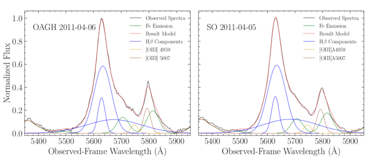
Fig 1 Example of spectral decomposition for the Hβ region in the 3C 273 spectra (observed frame) Left Panel: Spectra from the SO database. Right Panel: Spectra taken within 24 hours of each other. The color figure can be viewed online.
All measurements in this paper were made using the [O III], λ5007 Å emission line, in the observed frame; at the redshift of 3C 273, the line is at 5798 Å. This line is produced in the narrow-line region (NLR), and due to its large size, it is not expected to change over large periods of time, because the ionizing radiation will respond more slowly (Shapovalova et al. 2001, and references therein). Previous studies of IDV on 3C 273 mainly focus on the high-energy and optical bands and have not been reported for narrow lines. However, as mentioned earlier we do not expect such fast variations in narrow emission lines. An example of the low expected variations in these lines is presented in Yuan et al. (2022), where they calculate the [O III] λ5007 Å emission line flux. The variation between each day was always less than the uncertainties that could be obtained from the spectra. Additionally, for each pair of spectra, if the multi-Gaussian model was not fitted with similar amplitudes (taking into account that the width changes), then the spectra pair was discarded to avoid possible IDV.
From all the measurements obtained, we estimate the intrinsic profile and their uncertainty with error propagation for each quasi-simultaneous observation. Assuming that the intrinsic profiles for each date on the spectra of both observatories are the same (since they are quasi-simultaneous), we were able to estimate the instrumental broadening of the SO spectra, using the intrinsic profile widths obtained from OAGH and OAN-SPM, and the observed profile widths measured in the SO spectra. We estimated a weighted mean for the instrumental broadening measurements of the two slit widths available and calculated the standard error of the weighted mean.
4. Results
This analysis shows us that the instrumental profile for the SO spectra for the slit widths of 5.1, and 7.6 arcsec are 16.55 ± 4.43, and 23.23 ± 1.79Å, respectively. Given that the instrumental broadening should be proportional to the slit width, we can take any of the instrumental broadening measurements we have and obtain expected values for the instrumental profiles of the other slit widths. This means that for any two slit widths (e.g. a and b) these values must satisfy FWHM inst (a)/FWHM inst (b) = SW(a)/SW(b). For example, for the slit width of 4.1 (that we do not measure) and 7.6 (that we do measure), the instrumental broadening for the former is calculated as FWHM4.1 = FWHM7.6 × 4.1/7.6.
Since we have two measurements of the instrumental broadening, we obtained two sets of expected instrumental profiles, with their uncertainties, for all the slit widths. The difference between the values obtained for each slit width is most likely due to the uncertainties. We then calculated the mean of these two values for each slit width as well as their errors. These different values of instrumental broadening for each slit width are presented in Table 1.
TABLE 1 INSTRUMENTAL BROADENING FOR EACH SLIT WIDTH OF THE SPOL AT THE SO
|
|
Instrumental Broadening (Å) | ||
|---|---|---|---|
| Expected Values | Final Values | ||
| From 5.1 arcsec | From 7.6 arcsec | ||
| 2.0 | 6.49 ± 1.74 | 6.11 ± 0.47 | 6.30 ± 1.80 |
| 3.0 | 9.74 ± 2.61 | 9.17 ± 0.71 | 9.45 ± 2.70 |
| 4.1 | 13.31 ± 3.57 | 12.53 ± 0.97 | 12.92 ± 3.69 |
| 5.1 | 16.55 ± 4.44 | 15.59 ± 1.20 | 16.07 ± 4.59 |
| 7.6 | 24.67 ± 6.61 | 23.23 ± 1.79 | 23.95 ± 6.85 |
| 12.7 | 41.22 ± 11.04 | 38.82 ± 2.99 | 40.02 ± 11.44 |
In Figure 2, left panel we present the instrumental broadening obtained through this analysis for the spectra taken with slit widths of 5.1 and 7.6 (red diamonds), and the expected values estimated with both measurements (blue squares and orange circles respectively). The final instrumental broadening values for all the slit widths (green circles) are presented in Figure 2 right panel.
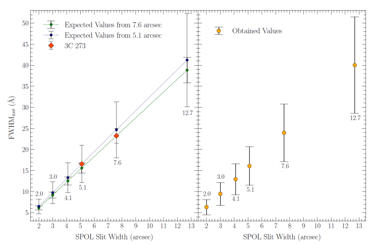
Fig. 2 Left panel: Expected sets of instrumental profiles with their uncertainties, measured using a 5.1 arcsec (navy blue squares and dotted line), and a 7.6 arcsec (orange dots and dashed line) slit width as a reference point. Observational measurements of instrumental broadening are also shown (red diamonds). Right panel: Instrumental broadening estimations for all 6 slit widths based upon the mean of the two expected values for each slit width. The color figure can be viewed online.
5. Conclusions
We have estimated the instrumental broadening for the six different slit widths used in the spectroscopic observations carried out by the Steward Observatory8, and the results are presented in Table 1. Notably, there is a significant difference in instrumental broadening across the different slit widths (which is expected), with the ratio between the maximum and minimum broadening being approximately 6.35 times. This highlights the importance of considering distinct instrumental broadening values for each slit width. Using a fixed or mean instrumental broadening for all slit widths will lead to an overestimation for smaller slit widths and an underestimation for the larger ones. Even when using mean and root mean square (rms) spectra with multiple slit widths, it is not correct to use a single instrumental broadening value, because the resulting spectra would still retain broadening information from all the slit widths, and they are strongly dependent on the most used setup.

