2.1. Observations

We carry out Johnson U BV observations of the target stars with a 0.35m Schmidt-Cassegrain telescope equipped with Optec SSP-5 photometer located at Ege University Observatory Application and Research Center (EUOARC). The photometer includes an R6358 photomultiplier tube, which is sensitive to the longer wavelengths at the optical part of the electromagnetic spectrum. We use a circular diaphragm with an angular size of 53^′′ and we adopt ten seconds of integration time for all observations. A typical observing sequence for a selected target is like sky-sky-VAR-VAR-VAR-VAR-sky-sky, where sky and VAR denote measurements from the sky and the variable star, respectively. We list the target stars in Table 1.

We follow the procedure described in ^{Hardie (1964)} to obtain reduced instrumental magnitudes. Moreover, we observe a set of standard stars selected from ^{Landolt (2009)} and ^{Landolt (2013)} along with each target. Hence, we transform all reduced instrumental magnitudes of the target stars into the standard system. Since RA coordinates of the target stars are distributed homogeneously around the celestial equator, we carried out standard star observations on two nights with an almost six-month time difference. These are 27th December 2022 and 13th July 2023 nights. We give computed transformation coefficients in the Appendix section.

Preliminary analysis of the EUOARC observations shows that signal-to-noise ratios of TYC 5275-00646-1, V1330 Sco, TYC 5610-00066-1, TYC 5050-00802-1, TYC 01572-00794-1 and GSC 00140-01925 are not sufficient for reliable colour and magnitude measurements. Increasing the integration time or gain, or using another EUOARC telescope (0.4m Schmidt-Cassegrain with a CCD camera and standard Johnson-Bessell filters) does not change the situation. Therefore, we take B − V colours and V magnitudes of these stars from The AAVSO Photometric All-Sky Survey for analysis (APASS; ^{Henden et al. 2015}). We tabulate standard colours and magnitudes of the target systems in Table 2.

2.2. Long-Term Photometry

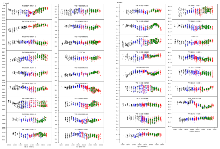
Besides EUOARC observations, we collect long-term V photometry of target stars from The All Sky Automated Survey (ASAS, ^{Pojmanski 1997}, ²⁰⁰²; ^{Pojmanski et al. 2005}) and All-Sky Automated Survey for Supernovae Sky Patrol (ASAS-SN, ^{Shappee et al. 2014}; ^{Kochanek et al. 2017}). The time range of the collected data usually spans over 15 or 18 years, depending on the beginning and the end of the observations. However, there is a significant time gap (3 or 4 years) between ASAS and ASAS-SN data, where no observation is available. This prevents us from precise tracing of the long-term photometric behaviour of our target systems. These time gaps are filled with unpublished observations obtained in the scope of the extension of the ASAS project (ASAS3-N and ASAS4; Pojmanski, 2022; priv. comm.). Therefore, we are able to collect photometric data of the target stars without a significant time gap. We plot the collected data of each target in Figure 1.

Fig. 1 Compiled ASAS3 (black), ASAS3-N (blue), ASAS4 (red) and and ASAS-SN (green) photometry of target stars. The colour figure can be viewed online. 

3.1. Photometric Properties

In the first step of our analysis, we plot measured standard U − B and B − V colours of the target systems in a colour - colour diagram (Figure 2). More than half of the target stars appear systematically shifted from the predicted positions of the unreddened main sequence stars. This could be interpreted as the effect of interstellar reddening, which means a kind of systematic interstellar reddening is valid for most of our target stars. However, these stars are located at different positions in the celestial sphere. If one applied a reddening correction suggested by Figure 2, then many of the target stars would become early-type stars. This is contradictory to the reported properties of our target stars, such as detected X-ray emission, photometric colours and light curve properties (see references mentioned in Table 1). In this case, interstellar reddening cannot be a satisfactory explanation for the disagreement between observed and predicted colours seen in Figure 2. An alternative explanation is colour excess due to the chromospheric activity of the target stars. Since their chromospheric activity was confirmed by their properties in the references mentioned above, we may expect average colour excesses of 0.m09 and 0.m35 for B − V and U − B colours, respectively (^{Amado 2003}). Due to these colour excesses, the observed U − B and B − V colours become bluer than their predicted values from standard stellar atmosphere models. An observational test of the suggested colour excess was done for the observed colours of HD 208472, an RS CVn variable, and corrected colours indicated an effective temperature, which was in agreement with spectroscopically estimated one (^{Özdarcan et al. 2010}). To calculate reliable astrophysical parameters of the target stars, we aim to remove the effects of both interstellar reddening and activity-originated colour excess from the observed B − V colours. Regarding interstellar reddening, we adopt the estimated mean E(B − V) colour excess (^{Schlafly & Finkbeiner 2011}) for the precise equatorial coordinates of each target. Then, we subtract the estimated E(B − V) excess from the observed B − V colour (fourth column in Table 2). For correction of activity-originated average blue excess in B − V colour, we add 0.09.m to each reddening corrected B − V colour and obtain the final B − V colour index of each target. We list the estimated E(B − V) values and corrected B − V ₀ colour index of each target in the last two columns of the Table 2. Here, we note that we find unreasonably large reddening for V1330 Sco (E(B − V) ≈ 1.m88) from ^{Schlafly & Finkbeiner (2011)}. Using this correction, we find a hot (≈ 25000 K) main sequence star. This finding is not consistent with the previously reported properties of the star (see reference given in Table 1). Therefore, we omit the effect of interstellar reddening for this star and only apply the activity-related 0.m09 colour excess correction to the observed B − V colour index.

Fig. 2 Positions of the target systems on the U BV colour - colour diagram. Six targets that do not have reliable measurements are not plotted in the figure. The continuous curve (black) shows the theoretically expected positions of the unreddened main sequence stars, while the dashed curves show the positions of unreddened giant (shorter curve) and supergiant stars (longer curve), respectively. The dashed (black) line denotes the reddening vector. Theoretical data are from ^{Drilling & Landolt (2000)}. The colour figure can be viewed online. 

3.2. Astrophysical Properties

By using the corrected B −V colours, we first determine the effective temperatures (T _{ef f} ) and bolometric corrections (BC) of the target stars according to the empirical colour - temperature and colour - bolometric correction relations given in ^{Gray (2005)}. Then, we determine the distance of each target depending on its parallax measurement taken from the third GAIA data release (^{Gaia Collaboration et al. 2016}, ²⁰²³). In the third step, we use the measured magnitudes (in Table 2) and the calculated distances (d) of each target in the distance modulus formula and find the absolute V magnitude (M _V ). After that, we apply estimated bolometric corrections to the calculated M_V magnitudes and obtain the bolometric absolute magnitude (M _bol ) of each star. In the final step, we use the calculated M _bol of each star with the solar M _bol value of 4.m74 in Stefan-Boltzmann law and calculate the luminosity (L/L _⊙) of the target stars. We estimate the spectral classification of each star by comparing estimated effective temperatures and calculated luminosities with the calibrations given in ^{Gray (2005)}. Following the outlined procedure, we calculate the results listed in Table 3.

Now, we are in a position to determine the location of each target on the Hertzsprung - Russell (HR) diagram (Figure 3). In the figure, one may notice that there is no available evolutionary track for the positions of a few targets located at the redder part of the diagram. These targets may be premain sequence stars, which still evolve towards the zero-age main sequence. LN Eri, V1330 Sco, V2700 Oph and KZ Psc might be premain sequence stars with their remarkably short photometric periods (P < 8 day) and a light curve amplitude between 0.m1 or 0.m 2 in the V filter (see Table 5 in the Appendix). Optical spectroscopic observations of these particular targets are required to arrive at a conclusive result.

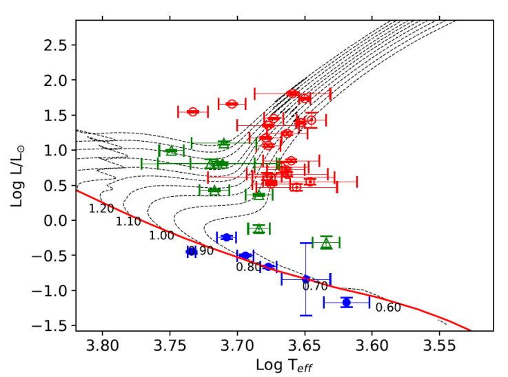
Fig. 3 Positions of the target systems on the HR diagram. Theoretical evolutionary tracks (dashed lines) for solar abundance (Y = 0.279 and Z = 0.017) are from ^{Bressan et al. (2012)}. Each track is labelled with its corresponding mass in solar units. Continuous (red) curve denotes the zero-age main sequence. Filled (blue) circles are for main sequence stars, open triangles (green) denote sub-giant stars and open (red) circles show giant stars. The colour figure can be viewed online. 

3.3. Analysis of Seasonal Light Curves

We use long-term photometry of each star (Figure 1) to determine seasonal light curve properties, which are photometric period (P _phot ), peak-to-peak light curve amplitude (A) and minimum (V _min ), maximum (V _max ) and mean (V _mean ) brightnesses. For that purpose, we first divide the photometric data of a given target into subsets, where each one covers an observing season. Then, we check each season by eye for any dramatic change in light curve amplitudes. If there is a significant amplitude change in a season, we further divide the corresponding subset into parts so that each part possesses a fairly constant amplitude.

Among photometric period determination methods, we employ Analysis of Variance (ANOVA, ^{Schwarzenberg-Czerny 1996}), which is a hybrid method that combines the power of Fourier analysis and ANOVA statistics. The method is capable of determining the best-fitting period for a given light curve independently of the shape of the light curve and is very effective to damp the amplitudes of the alias periods². To estimate the uncertainty of the computed photometric periods, we follow the method proposed by ^{Schwarzenberg-Czerny (1991)}. The method provides more accurate uncertainties compared to the least-squares correlation matrix or Rayleigh resolution criteria.

Before proceeding with the ANOVA method, we apply a linear fit to the corresponding subset light curve to remove any long-term brightness variation, because such a variation may alter the photometric period artificially. After the linear correction, we apply the ANOVA method to the residuals from the linear fit and determine the best-fitting period and the light curve properties mentioned above. After we find the final photometric period for a given subset, we make a phase-folded light curve of this subset concerning the final photometric period and fit a cubic spline polynomial to the phase-folded data. Here, the purpose is to determine the minimum and the maximum values of the spline function, which correspond to the brightnesses of the light curve maximum and minimum, respectively. The amplitude and the mean brightness can be calculated straight-forwardly from these values. Otherwise, fitted spline polynomials do not have any physical meaning. We list the analysis results in the Appendix (Table 5).

3.4. Photometric Periods and Surface Differential Rotation

In this section, we use the advantage of having long-term photometry to estimate the magnitude of the SDR. It is clear that determining the latitude of the cool surface spots from photometry is a well-known ill-posed problem. This prevents the type of differential rotation (solar type or anti-solar type) from being clearly determined in this study. However, the range in which the photometric period takes value for a particular star can set a lower limit for the magnitude of the SDR. Given the brief discussion above, we implicitly assume that all target stars possess solar-type SDR (i.e., the equator rotates faster than the poles). Therefore, we consider the observed minimum value of the photometric period as the equatorial rotation period. The observed maximum value, then, corresponds to the highest latitude at which spots could emerge during the time interval of the photometric data. We make a quantitative estimation of the magnitude of the SDR by relative shear defined in terms of periods (Equation 1),

We take P _max and P _min values of each target star from Table 5 and compute the relative shear via Equation 1. We plot the P _min - relative shear pair of each star in Figure 4. We also tabulate these pairs along with the estimated spectral types in Table 4.

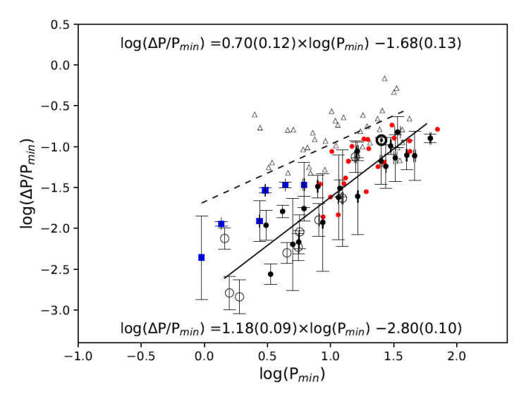
Fig. 4 Relation between the observed minimum period P _min and the calculated relative shear. Black filled circles show giant stars listed in Table 5, while blue filled square and open circle symbols denote main sequence stars and sub-giant stars, respectively. Open triangles show stars taken from ^{Donahue et al. (1996)}, small (red) dots (without error bars) show RS CVn stars analysed in ^{Özdarcan (2021)} and five other stars mentioned in the text. We also show the position of our Sun in the figure. Dashed and straight lines show linear fits to the distribution of main sequence and giant stars, respectively. The corresponding coefficients and their statistical errors are given inside the plot window (upper one for the main sequence stars, lower one for the giant stars). The colour figure can be viewed online. 

For comparison, we also show the positions of the 37 main sequence stars analysed in ^{Donahue et al. (1996)} and 21 giant stars analysed in ^{Özdarcan (2021)}. Five more giant stars are also plotted in the figure (with red dots), which are HD 208472 (^{Özdarcan et al. 2010}), FG UMa (HD 89546, ^{Ozdarcan et al. 2012}) and BD+13 50000, TYC 5163-1764-1 and BD+11 3024 (^{Özdarcan & Dal 2018}). We note that analysis of all these stars was done in a similar way as described above. The only difference could be that ^{Donahue et al. (1996)} used the S index based on Ca II H& K measurements, which is a spectroscopic indicator of the chromospheric activity. For the remaining stars, pure V photometry, which is a photometric indicator of the same phenomenon, was used.

A linear fit to the positions of all main sequence stars plotted in Figure 4 gives the coefficients shown in the upper part of the figure with a correlation coefficient of 0.67 and a p value of 6.9 × 10⁻⁷. In the figure, sub-giants and giants appear as aligned on the same slope. Thus, we apply a similar linear fit to the positions of all giant and sub-giant stars. The fit results in the coefficients shown in the bottom part of the figure with a correlation coefficient of 0.88 and a p value of 3.2 × 10⁻¹⁹.