


 nueva página del texto (beta)
 Inglés (pdf)
 Artículo en XML
 Referencias del artículo
 Enviar artículo por email
 Citado por SciELO
  Similares en
SciELO
Similares en
SciELO 
 Permalink
1 INTRODUCTION
The stellar trapezia are formed in the interior of emission nebulae, such as the Orion Nebula. They are physical systems formed by three or more approximately equal stars, where the largest separation between its stars is never larger than three times the smallest separation [Ambartsumian(1955)]. That means the distances between the stars that form a trapezium are of the same order of magnitude. Trapezia are completely different to the hierarchical systems, where there could be a difference of an order of magnitude (10) between the smallest and largest separations.
The best known trapezium system is found in the Orion Nebula. Figure 1 shows this prototypical system. The brightest star in this system is
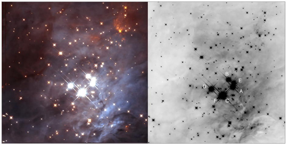
Fig. 1 The prototypical trapezium type system in the Orion Nebula. On the right, the six main components are marked (Taken from Allen et al. 2019). The colour figure can be viewed online.
Trapezia are not dynamically stable, the orbits of their stellar components are not closed. This leads very quickly to close encounters which result in the expulsion of one or more members of the system and by this they turn into hierarchical systems [Abt &Corbally(2000)]. As a consequence of this fact it is found that the maximum age of stellar trapezia cannot be larger than a few million years.
Using numerical simulation, Allen et-al.(2018) showed that stellar trapezia evolve in time in different ways according to their initial configuration; some systems could break up into individual stars, whilst others evolve into binary or more complex stellar systems.
The age and evolution of trapezia also help us understand the evolution of stars. Knowing the distance between their stars and the total size of a trapezium system is fundamental in order to understand its dynamical evolution Abt(1986).
This paper constitutes the first part of a photometric, spectroscopic and dynamical study of trapezia in our Galaxy. In § 2 we present the observations of the standard stars as well as those of the stars in the trapezia, in § 3 we discuss the slope of the reddening line on the two-colour diagram, and in § 4 we present our conclusions.
2 The Observations
The observations were performed during two observing seasons in June and December 2019, with the 84 cm telescope at the OAN in San Pedro Mártir, Baja California, México. We observed regions of standard stars Landolt(1992) in the five filters of interest (U-I) distributed along the night so as to have measurements at different values of air mass. Interspersed within these observations, we observed the stars in the trapezia of interest. The images have a plate scale of
2.1 Reduction of Standard Stars
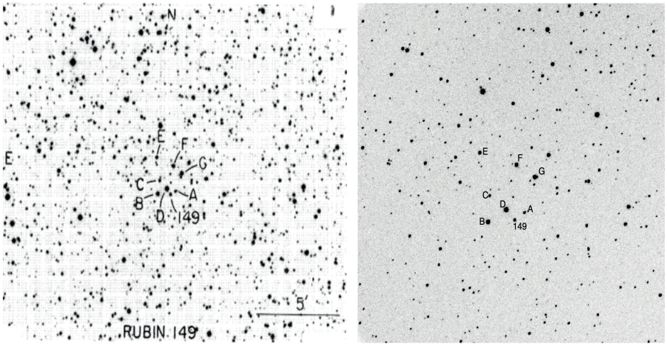
The standard stars are used in general to calibrate other astronomical observations. In this work, we shall refer to the set of equatorial standard stars published by [Landolt(1992)]. We observed several of the Landolt standard regions every night and used them to calibrate our observations of the trapezia stars. Figure 2 shows a comparison of the standard region Rubin 149 observed by [Landolt(1992)] and by us.
In order to express the magnitude of the stars in the trapezia in a standard system, we performed aperture photometry of stars in some of the Landolt Standard Regions [ Landolt(1992)]. The photometric measurements of the standard stars were carried out using the APT (Aperture Photometry Tool) programme, (see https://www.aperturephotometry.org/about/), and Laher et-al.(2012).
The APT programme is a software that permits aperture photometry measurements of stellar images on a frame. The programme accepts images in the fits format; therefore, no transformation of the images to other formats was necessary. The observed standard regions had already been pre-processed.
The transformation equations between the observed and intrinsic photometric systems are as follows:
where the suffixes int and obs stand for intrinsic and observed. The coefficients A, K and C represent the negative of the coefficient of atmospheric absorption, a colour term and a zero point shift term. We intend to calculate these terms using the observed values measured with APT, and the intrinsic values for the magnitudes given in [Landolt(1992)]. The least squares procedure is used to solve the equations, and the coefficients obtained are shown in Tables 1-5.
Table 1: Transformation Coefficients for U
| Standard Systems | A | K | C |
|---|---|---|---|
| 13-14 June 2019 | -0.56 | 0.13 | 23.51 |
| 10-11 December 2019 | -0.44 | 0.18 | 23.49 |
| 12-13 December 2019 | -1.20 | 0.06 | 24.47 |
| 13-14 December 2019 | - | - | - |
| 14-15 December 2019 | 17.07 | -85.51 | 46.00 |
| 15-16 December 2019 | -0.49 | 0.14 | 23.60 |
Table 2: Transformation Coefficients for B
| Standard Systems | A | K | C |
|---|---|---|---|
| 13-14 June 2019 | -0.28 | 0.04 | 25.42 |
| 12-11 December 2019 | -0.26 | 0.04 | 25.39 |
| 12-13 December 2019 | -0.30 | 0.02 | 25.40 |
| 13-14 December 2019 | 664.84 | 3.79 | -693.02 |
| 14-15 December 2019 | -0.14 | -0.08 | 25.14 |
| 15-16 December 2019 | -0.31 | 0.04 | 25.42 |
Table 3: Transformation Coefficients for V
| Standard Systems | A | K | C |
|---|---|---|---|
| 13-14 June 2019 | -0.17 | -0.07 | 25.04 |
| 10-11 December 2019 | -0.14 | -0.07 | 25.05 |
| 12-13 December 2019 | -0.10 | -0.08 | 24.97 |
| 13-14 December 2019 | -39.46 | 0.75 | 63.66 |
| 14-15 December 2019 | -0.14 | -0.09 | 25.04 |
| 15-16 December 2019 | -0.17 | -0.06 | 25.10 |
Table 4: Transformation Coefficients for R
| Standard Systems | A | K | C |
|---|---|---|---|
| 13-14 June 2019 | -0.14 | -0.05 | 25.09 |
| 12-11 December 2019 | -0.10 | -0.07 | 25.16 |
| 12-13 December 2019 | -0.14 | -0.03 | 25.15 |
| 13-14 December 2019 | 19.33 | -2.21 | 5.28 |
| 14-15 December 2019 | -0.09 | -0.07 | 25.10 |
| 15-16 December 2019 | -0.19 | -0.07 | 25.22 |
Table 5: Transformation Coefficients for I
| Standard Systems | A | K | C |
|---|---|---|---|
| 13-14 June 2019 | -0.10 | 0.11 | 24.95 |
| 10-11 December 2019 | -0.04 | 0.11 | 25.06 |
| 12-13 December 2019 | -0.34 | 0.14 | 25.47 |
| 13-14 December 2019 | -3.51 | -1.37 | 29.93 |
| 14-15 December 2019 | -0.06 | 0.07 | 25.11 |
| 15-16 December 2019 | -0.12 | 0.05 | 25.17 |
In Figure 3 we see graphs of the calculated magnitude minus the intrinsic magnitude versus the observed instrumental magnitude
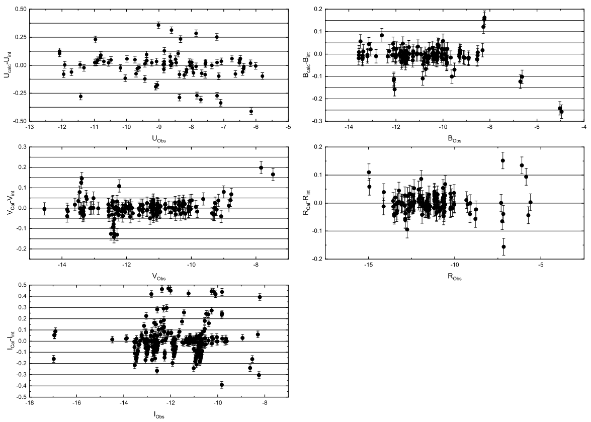
Table 6: Measured counts for components A to F of ADS 13292, obtained with AstroImageJ and APT
| Number of Counts (AstroImageJ) |
Number of Counts (APT) |
Difference (counts) |
Difference(%) (Percentage) |
|
|---|---|---|---|---|
| A | 163657.5663 | 163640 | 17.566316 | 0.01073358012 |
| B | 1505427.035 | 1503700 | 1727.034662 | 0.1147205824 |
| C | 72591.87383 | 72488.6 | 103.273825 | 0.1422663716 |
| D | 58946.5638 | 59003 | 56.436205 | 0.09574129748 |
| E | 123743.0788 | 123762 | 18.921178 | 0.015290696 |
| F | 1170320.58 | 1169260 | 1060.580108 | 0.09062304176 |
|
|
|
|
|
|
| A | 40307.63323 | 40359.5 | 51.866766 | 0.1286772798 |
| B | 94842.91829 | 94752.7 | 90.218291 | 0.0951239087 |
| C | 871463.4746 | 870522 | 941.474566 | 0.1080337379 |
| D | 80068.28323 | 80192.9 | 124.616769 | 0.1556381178 |
| E | 150244.2993 | 150189 | 55.299313 | 0.0368062637 |
| F | 1175990.939 | 1175830 | 160.93914 | 0.01368540646 |
2.2 Photometry of Trapezia Stars
Trapezia are open clusters in which their stars interact gravitationally, and this interaction has very noticeable dynamical consequences. As mentioned in subsection 2.1 the aperture photometry for the standard stars was done using the APT programme. However, the photometry of the trapezia stars must be carried out on a set of more than a thousand images. For this photometric measurements, we used the aperture photometry capabilities of the programme AstroImageJ (see http://astro.phy.vanderbilt.edu/vida/aij.htm, [Collins et-al.(2017). As the aperture photometry measurements carried out with AstroImageJ are automatic, we performed a comparison between the results obtained with APT and with AstroImageJ for the stars in one trapezium. Table 7 shows a comparison between the number of counts obtained with AstroImageJ and that found with APT. This was done for measurements of the six components (A, B, C, D, E, and F) of the trapezium ADS 13292; the full photometry for this trapezium will be reported elsewhere. As stated in the last column of this table, the difference in the number of counts measured with one programme or the other is at most of the order of 0.1%.
Table 7: Photometric aperture radii in pixels for the trapezium ADS 15184
| r1 (pix) | r2 (pix) | r3 (pix) | |
|---|---|---|---|
| AB | 8 | 12 | 16 |
| C | 8 | 11 | 14 |
| D | 8 | 11 | 14 |
We opted for using the AstroImageJ programme for the measurement of the stellar components of the different trapezia since the measurement of a large number of images may be done in an automatic way.
2.2.1 ADS 15184
The trapezium ADS 15184 (also known as WDS 21390+5729) is located at RA=21h 38m, Dec=+57° 29. It has four bright components denoted as A, B, C, and D. Their distribution is presented on the left of Figure 4. The right panel of this figure shows our image for ADS 15184 in the V filter. On the figure we have identified the components A, B, C and D. The A and B components are very bright and even on the short time exposure appear melded as shown in Figure 5. Due to this fact, the photometry of both these objects is carried out as if they represented one star only, which we denote as the AB component.
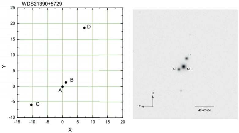
Fig. 4 The left image represents the components of the trapezium ADS 15184. The axes are given in arcsecs. On the right, we show our observed image in the V filter, with N-E orientation and scale in arsecs. Exposure time is 0.2 seconds
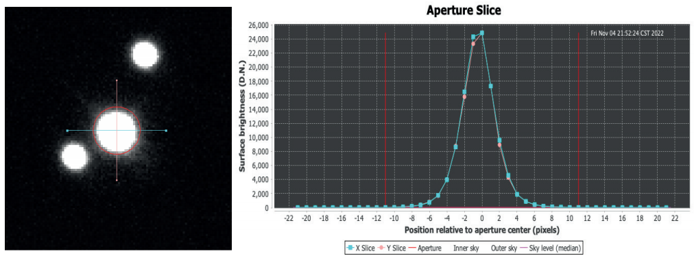
Fig. 5 At the centre of the left image we show the blended AB components of ADS 15184. On the right panel, vertical and horizontal cuts are performed on the central star component AB. These cuts show that components A and B are not well resolved in our images. The colour figure can be viewed online.
We obtained 70 images of this trapezium in the filters U - I. Two sets of images were taken with integration times of 0.1 and 8 seconds respectively, so that we could get images where the bright stars were not saturated and also images where the fainter stars could have a substantial number of counts.
To perform photometry on each one of the stars of a trapezium, it is necessary to vary the aperture radius to ensure that the same percentage of the light is included for each stellar image. Table 7 shows the radii for each component, where r 1 is the radius of the central aperture, r 2 is the inner radius of the sky annulus, and r 3 is the outer radius of the sky annulus.
The photometric measurements we obtained are given in number of counts, which is directly proportional to the exposure time. We normalise all our measurements to a standard time of 10 seconds. To achieve this, we use the following equation:
Where I 10 represents the intensity of the star at the normalised time (10 seconds), t is the observation time and I obs is the observed intensity. The normalised intensity is transformed to magnitude in a standard manner.
Using equations 1-5 for each filter and taking the coefficients A, K and C for the night 10 - 11 December, shown in Tables 1-5, we calculate the values for the magnitudes and colours of the stars in the trapezium. We estimate the magnitude errors to be of the order of
Table 8: Observed Magnitudes and Colours for the stars in trapezium ADS15184
| U | B | V | R | I | U - B | B - V | V - R | R - I | V - I | |
|---|---|---|---|---|---|---|---|---|---|---|
| AB | 5.29 | 5.62 | 5.37 | 5.28 | 5.10 | -0.33 | 0.24 | 0.09 | 0.18 | 0.27 |
| C | 7.93 | 8.18 | 7.87 | 7.66 | 7.49 | -0.25 | 0.32 | 0.20 | 0.17 | 0.37 |
| D | 7.83 | 8.05 | 7.80 | 7.67 | 7.52 | -0.22 | 0.25 | 0.13 | 0.15 | 0.28 |
Using the colour values, we may determine the Q index (see Johnson & Morgan (1953)), which we know is reddening independent:
We can associate a different spectral type to different values of Q depending on whether we consider stars of Luminosity Class I (Supergiants) or V (Dwarfs) (see Table 9). We could also use for this classification the empirical calibration published by [Lyubimkov et-al.(2002) in which they associate the effective temperature of stars of luminosity classes II-III and IV-V to the value of the Q-parameter (see their equations 6 and 7 and their Figure 11). We shall try this approach elsewhere.
Table 9: Q versus Spectral Type. Taken from Johnson & Morgan (1953)
| Spectral Type | Q | Spectral Type | Q |
|---|---|---|---|
| O5 | -0.93 | B3 | -0.57 |
| O6 | -0.93 | B5 | -0.44 |
| O8 | -0.93 | B6 | -0.37 |
| O9 | -0.9 | B7 | -0.32 |
| B0 | -0.9 | B8 | -0.27 |
| B0.5 | -0.85 | B9 | -0.13 |
| B1 | -0.78 | A0 | 0 |
| B2 | -0.7 |
Table 10 gives the spectral types associated to each star of this trapezium based on the values of Q. In the case of AB, the spectral type given is that of a star that results from the union of A and B.
From the U - B and B - V colours shown in Table 9 we make a two-colour diagram, where the red dots represent the components AB, C and D. The blue and green lines represent the intrinsic main sequence and the intrinsic supergiant sequence respectively. We also see the reddening line (red colour line, see Figure 6). This line has a slope equal to
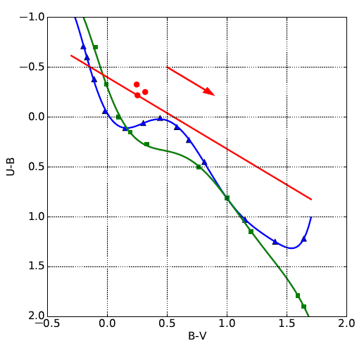
Figure 6: Two colour diagram (U - B vs B - V) for ADS 15184. The green line is the supergiant intrinsic sequence (SGIS), in blue the main sequence (MSIS) intrinsic sequence and the red dots represent the observed colours of the components of this trapezium. The red line and the red arrow represent the reddening line and direction. The colour figure can be viewed online.
Finding the intersection of a line parallel to the reddening line that also passes on the observed points with the intrinsic sequences allows us to find the intrinsic colours of each star, which permits us to calculate the colour excess E (B - V), the absorption A
V
and the distance in parsecs to the star in question (
Table 11gives the values for the intrinsic colours, the excesses, the absorption and distances assuming the stars are supergiants (top panel), while in the bottom panel it gives the same information assuming the stars belong to the main sequence.
Table 11: Intrinsic colours, colour excess, absorption and distance for ADS 15184
| Assuming Supergiant Stars | |||||||
|---|---|---|---|---|---|---|---|
| (U - B)0 | (B - V)0 | EU - B | EB - V | AV | Distance (pc) | Parallax (mas) | |
| AB | -0.56 | -0.07 | 0.23 | 0.32 | 0.99 | 1380.43 | 0.72 |
| C | -0.53 | -0.07 | 0.27 | 0.38 | 1.18 | 3975.93 | 0.25 |
| D | -0.43 | -0.04 | 0.21 | 0.29 | 0.90 | 4349.30 | 0.23 |
| Assuming Main Sequence Stars | |||||||
| (U - B)0 | (B - V)0 | EU - B | EB - V | AV | Distance (pc) | Parallax (mas) | |
| AB | -0.63 | -0.18 | 0.31 | 0.42 | 1.31 | 135.51 | 7.38 |
| C | -0.60 | -0.17 | 0.35 | 0.49 | 1.51 | 389.58 | 2.57 |
| D | -0.51 | -0.15 | 0.29 | 0.40 | 1.24 | 355.85 | 2.81 |
A comparison of our results with the SIMBAD Astronomical Database [Wenger et-al.(2000) is presented in Table 13. The magnitudes of the stars listed in SIMBAD come from the following references: [Fabricius et-al.(2002), [Reed(2003)], [Mercer et-al.(2009), and [Zacharias et-al.(2012). Table 12 shows that our magnitudes differ in the worst case by one magnitude.
Table 12: Comparison of our measurements of ADS 15184 with SIMBAD (*)
| Magnitude | |||
|---|---|---|---|
| AB | C | D | |
| U | 5.29 | 7.93 | 7.83 |
| U * | - | 7.72 | 7.53 |
| B | 5.62 | 8.18 | 8.05 |
| B * | - | 7.63 | - |
| V | 5.37 | 7.87 | 7.80 |
| V * | - | 7.46 | - |
| R | 5.28 | 7.66 | 7.67 |
| R* | - | - | 8.73 |
| I | 5.10 | 7.49 | 7.52 |
| I * | - | 7.67 | - |
| Spectral Type | |||
| AB | C | D | |
| St | B5 | B5 | B6 |
| St* | - | B1.5V | B1V |
| Parallax | |||
| AB | C | D | |
| Psg | 0.72 | 0.25 | 0.23 |
| Psp | 7.38 | 2.57 | 2.81 |
| P* | - | 0.8589 | 1.1051 |
Table 13: Dereddened magnitudes and colours for stars in ADS 15184 using van de Hulst curve 15
| Assuming Supergiant Stars | ||||||||||
|---|---|---|---|---|---|---|---|---|---|---|
| U | B | V | R | I | U - B | B - V | V - R | R - I | V - I | |
| AB | 3.76 | 4.31 | 4.39 | 4.55 | 4.63 | -0.55 | -0.07 | -0.16 | -0.08 | -0.25 |
| C | 6.10 | 6.62 | 6.68 | 6.78 | 6.93 | -0.52 | -0.07 | -0.10 | -0.14 | -0.25 |
| D | 6.44 | 6.86 | 6.90 | 7.00 | 7.09 | -0.42 | -0.04 | -0.10 | -0.09 | -0.19 |
| Assuming Main Sequence Stars | ||||||||||
| U | B | V | R | I | U - B | B - V | V - R | R - I | V - I | |
| AB | 3.25 | 3.88 | 4.06 | 4.31 | 4.48 | -0.63 | -0.18 | -0.25 | -0.17 | -0.42 |
| C | 5.58 | 6.18 | 6.35 | 6.54 | 6.77 | -0.60 | -0.17 | -0.19 | -0.23 | -0.42 |
| D | 5.91 | 6.41 | 6.56 | 6.75 | 6.93 | -0.50 | -0.15 | -0.19 | -0.18 | -0.37 |
Using Curve 15 of van de Hulst’s [Johnson(1968)] we can obtain the dereddened values of the magnitudes for each component. The results of this exercise is shown in Table 15, these values coincide with those reported in Table 11.
2.2.2 ADS 4728
Trapezium ADS 4728 (also known as WDS 06085+13358) located at RA=6h 8m, Dec=+13°. 58 It has eleven components: A - K, which are distributed as shown on the left panel of Figure 7.
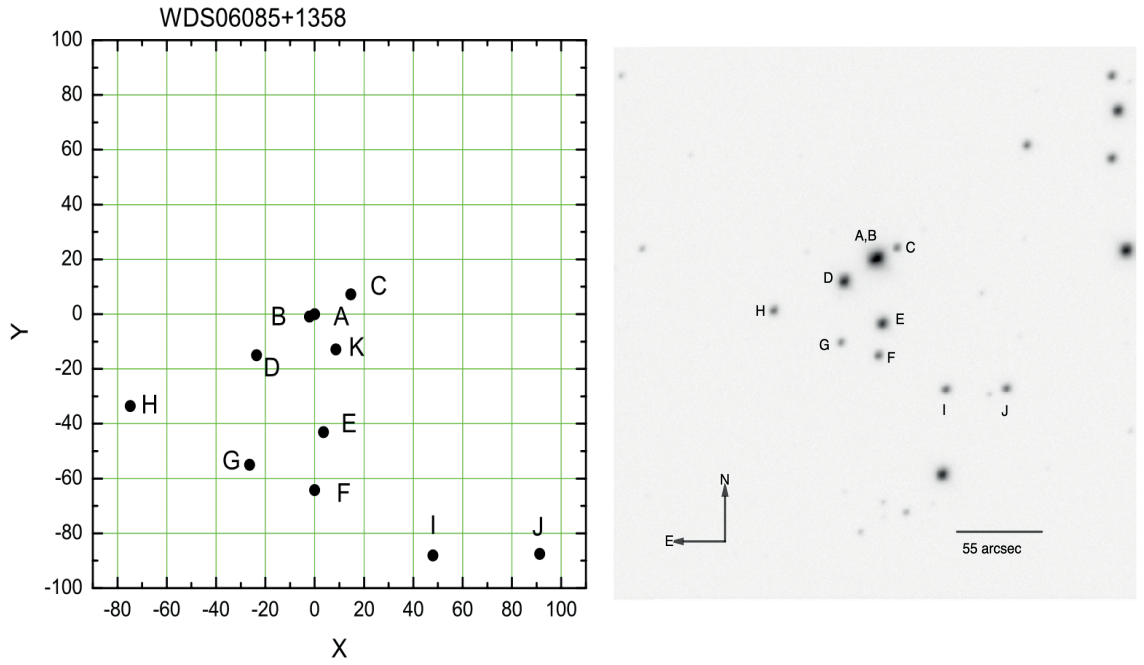
Fig. 7 The left image represents the components of the trapezium ADS 4728. The axes units are seconds of arc. On the right, we show our observed image in the V filter, with N-E orientation and scale in arsecs. Exposure time is 1 second.
We observed 110 images for this trapezium in filters U - I.
The images for this trapezium were obtained with three different integration times 0.5, 1 and 8 seconds.
Figure 7 also shows an image of this trapezium in the V filter (right panel). The stellar components as well as the orientation and plate scale are indicated on this figure.
Table 14 shows the values of the radii we used for performing the photometry for each component. As done previously, all the measurements are normalised to 10 seconds with Equation 6.
Table 14: Photometric aperture radii for ADS 4728
| r1 (pix) | r2 (pix) | R3 (pix) | |
|---|---|---|---|
| C | 9 | 11 | 13 |
| D | 10 | 11 | 14 |
| E | 9 | 11 | 14 |
| F | 9 | 11 | 14 |
| G | 11 | 13 | 16 |
| H | 11 | 13 | 16 |
| I | 10 | 12 | 14 |
| J | 10 | 12 | 14 |
Using the values of A, K and C we obtain the magnitudes and colours for the stars of trapezium ADS 15184 (see Table 15).
Table 15: Observed magnitudes and colours for trapezium ADS 4728
| U | B | V | R | I | U - B | B - V | V - R | R - I | V - I | |
|---|---|---|---|---|---|---|---|---|---|---|
| C | 11.66 | 11.72 | 11.51 | 11.46 | 11.31 | -0.05 | 0.21 | 0.04 | 0.15 | 0.20 |
| D | 7.98 | 8.60 | 8.59 | 8.64 | 8.62 | -0.62 | 0.01 | -0.05 | 0.02 | -0.03 |
| E | 8.88 | 9.22 | 9.12 | 9.13 | 9.04 | -0.35 | 0.10 | -0.00 | 0.08 | 0.08 |
| F | 11.16 | 11.08 | 10.87 | 10.83 | 10.68 | 0.08 | 0.21 | 0.04 | 0.15 | 0.19 |
| G | 12.11 | 11.98 | 11.76 | 11.72 | 11.57 | 0.13 | 0.22 | 0.04 | 0.15 | 0.18 |
| H | 12.25 | 11.08 | 9.88 | 9.34 | 8.76 | 1.17 | 1.21 | 0.54 | 0.58 | 1.12 |
| I | 10.70 | 10.87 | 10.75 | 10.74 | 10.65 | -0.17 | 0.12 | 0.01 | 0.09 | 0.09 |
| J | 10.72 | 10.95 | 10.81 | 10.76 | 10.64 | -0.22 | 0.13 | 0.05 | 0.12 | 0.17 |
Table 16 shows the spectral type associated to each star from the Q parameter calibration
Table 16: Q derived spectral types for ADS 4728
| Q | Spectral Type | |
|---|---|---|
| C | -0.20 | B8 |
| D | -0.63 | B3 |
| E | -0.42 | B5 |
| F | -0.08 | B9 |
| G | -0.03 | A0 |
| H | 0.30 | A0 |
| I | -0.26 | B8 |
| J | -0.32 | B7 |
Using the U - B and B - V colours from Table 15 we plot the points on the two-colour diagram (see Figure 8) where the same conventions as those followed for the previous trapezium are followed.
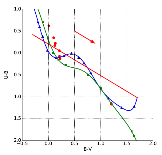
The first part of Table 17 presents the values for intrinsic colours, colour excesses, absorption and distances assuming the stars are supergiants, while the second part shows the same results assuming the stars to be in the main sequence.
Table 17 Intrinsic colours, colour excesses, Absorption and distances for ADS 4728
| Assuming Supergiant Stars | |||||||
|---|---|---|---|---|---|---|---|
| (U - B)0 | (B - V)0 | EB - V | EU - B | AV | Distance (pc) | Parallax (mas) | |
| C | -0.17 | 0.04 | 0.17 | 0.12 | 0.52 | 27948.93 | 0.04 |
| D | -0.71 | -0.11 | 0.12 | 0.09 | 0.38 | 8201.46 | 0.12 |
| E | -0.45 | -0.04 | 0.14 | 0.10 | 0.45 | 9945.13 | 0.10 |
| F | 0.00 | 0.11 | 0.10 | 0.07 | 0.32 | 22636.52 | 0.04 |
| G | 0.07 | 0.14 | 0.08 | 0.06 | 0.25 | 34886.01 | 0.03 |
| H | - | - | - | - | - | - | - |
| I | -0.25 | 0.02 | 0.11 | 0.08 | 0.33 | 21454.01 | 0.05 |
| J | -0.32 | -0.01 | 0.14 | 0.10 | 0.44 | 21340.38 | 0.05 |
| Assuming Main Sequence Stars | |||||||
| (U - B)0 | (B - V)0 | EB - V | EU - B | AV | Distance (pc) | Parallax (mas) | |
| C | -0.26 | -0.08 | 0.29 | 0.21 | 0.91 | 1466.26 | 0.68 |
| D | -0.78 | -0.21 | 0.22 | 0.16 | 0.69 | 1261.05 | 0.79 |
| E | -0.53 | -0.15 | 0.25 | 0.18 | 0.79 | 969.79 | 1.03 |
| F | -0.09 | -0.03 | 0.24 | 0.17 | 0.74 | 931.28 | 1.07 |
| G | -0.02 | 0.01 | 0.22 | 0.16 | 0.67 | 866.56 | 1.15 |
| H | - | - | - | - | - | - | - |
| I | -0.34 | -0.10 | 0.23 | 0.16 | 0.71 | 1132.09 | 0.88 |
| J | -0.41 | -0.12 | 0.26 | 0.18 | 0.80 | 1483.90 | 0.67 |
The magnitudes of the stars listed in SIMBAD come from the following references: [Høg et-al.(2000), [Zacharias et-al.(2003), [Reed(2003)], [Zacharias et-al.(2009), [Krone-Martins et-al.(2010), and [Gaia Collaboration (2020)]. Table 18 shows our results compared with those listed in SIMBAD (shown with *).
Table 18: Comparison of our results for ADS 4728 with SIMBAD (*)
| Magnitude | ||||||||
|---|---|---|---|---|---|---|---|---|
| C | D | E | F | G | H | I | J | |
| U | 11.66 | 7.98 | 8.88 | 11.16 | 12.11 | 12.25 | 10.70 | 10.72 |
| U* | - | 7.75 | - | - | 10.94 | - | - | - |
| B | 11.72 | 8.60 | 9.22 | 11.08 | 11.98 | 11.08 | 10.87 | 10.95 |
| B* | 11.51 | 8.239 | 9.051 | 11.02 | 11.882 | 11.03 | 10.82 | - |
| V | 11.51 | 8.59 | 9.12 | 10.87 | 11.76 | 9.88 | 10.75 | 10.81 |
| V * | 11.529 | 8.659 | 9.265 | 10.968 | 11.892 | 9.905 | 10.825 | - |
| R | 11.46 | 8.64 | 9.13 | 10.83 | 11.72 | 9.34 | 10.74 | 10.76 |
| R * | 11.32 | 8.89 | 9.10 | 10.86 | 11.69 | 9.65 | - | - |
| I | 11.31 | 8.63 | 9.04 | 10.68 | 11.57 | 8.76 | 10.65 | 10.64 |
| I* | - | - | - | - | 12.40 | - | - | - |
| Spectral Type | ||||||||
| C | D | E | F | G | H | I | J | |
| St | B8 | B3 | B5 | B9 | A0 | A0 | B8 | B7 |
| St* | B9V | B1V | B3V | B9V | - | G8 | B5 | - |
| Parallax | ||||||||
| C | D | E | F | G | H | I | J | |
| Psg | 0.04 | 0.12 | 0.10 | 0.04 | 0.03 | 0.24 | 0.05 | 0.05 |
| Psp | 0.68 | 0.79 | 1.03 | 1.07 | 1.15 | 10.27 | 0.88 | 0.67 |
| P* | 1.0671 | 0.96 | 0.9537 | 1.0783 | 1.0151 | 1.657 | 1. 086 | - |
Table 19 shows the dereddened values for magnitudes and colours for the stars in ADS 4728.
Table 19: Dereddened magnitudes and colours for ADS 4728 using van de Hulst curve 15
| Assuming Supergiant Stars | ||||||||||
|---|---|---|---|---|---|---|---|---|---|---|
| U | B | V | R | I | U - B | B - V | V - R | R - I | V - I | |
| C | 10.85 | 11.03 | 10.99 | 11.08 | 11.06 | -0.17 | 0.04 | -0.09 | 0.01 | -0.08 |
| D | 7.39 | 8.1 | 8.21 | 8.36 | 8.44 | -0.71 | -0.11 | -0.15 | -0.08 | -0.23 |
| E | 8.18 | 8.63 | 8.67 | 8.79 | 8.83 | -0.45 | -0.04 | -0.12 | -0.04 | -0.15 |
| F | 10.66 | 10.66 | 10.55 | 10.59 | 10.53 | 0 | 0.11 | -0.04 | 0.07 | 0.02 |
| G | 11.73 | 11.65 | 11.51 | 11.54 | 11.46 | 0.07 | 0.14 | -0.03 | 0.08 | 0.06 |
| H | 7.59 | 7.11 | 6.88 | 7.11 | 7.33 | 0.48 | 0.24 | -0.23 | -0.22 | -0.45 |
| I | 10.18 | 10.43 | 10.41 | 10.49 | 10.49 | -0.25 | 0.02 | -0.08 | 0 | -0.08 |
| J | 10.05 | 10.37 | 10.38 | 10.44 | 10.43 | -0.32 | -0.01 | -0.06 | 0.01 | -0.05 |
| Assuming Main Sequence Stars | ||||||||||
| U | B | V | R | I | U - B | B - V | V - R | R - I | V - I | |
| C | 10.26 | 10.52 | 10.6 | 10.79 | 10.88 | -0.26 | -0.08 | -0.19 | -0.09 | -0.28 |
| D | 6.91 | 7.69 | 7.9 | 8.13 | 8.29 | -0.78 | -0.21 | -0.23 | -0.16 | -0.39 |
| E | 7.65 | 8.18 | 8.33 | 8.54 | 8.67 | -0.53 | -0.15 | -0.21 | -0.13 | -0.33 |
| F | 10.02 | 10.11 | 10.14 | 10.28 | 10.33 | -0.09 | -0.03 | -0.15 | -0.04 | -0.19 |
| G | 11.07 | 11.09 | 11.09 | 11.22 | 11.25 | -0.02 | 0.01 | -0.13 | -0.03 | -0.17 |
| H | 6.77 | 6.41 | 6.34 | 6.71 | 7.07 | 0.36 | 0.06 | -0.37 | -0.36 | -0.73 |
| I | 9.6 | 9.93 | 10.04 | 10.22 | 10.31 | -0.33 | -0.1 | -0.18 | -0.1 | -0.28 |
| J | 9.49 | 9.89 | 10.02 | 10.17 | 10.26 | -0.4 | -0.12 | -0.15 | -0.09 | -0.24 |
2.2.3 ADS 2843
Trapezium ADS 2843 (also known as WDS 03541+3153) is at RA=3h 54m, Dec=+31° 53 and has five components: A, B, C, D, and E, distributed as seen on the left of Figure 9.
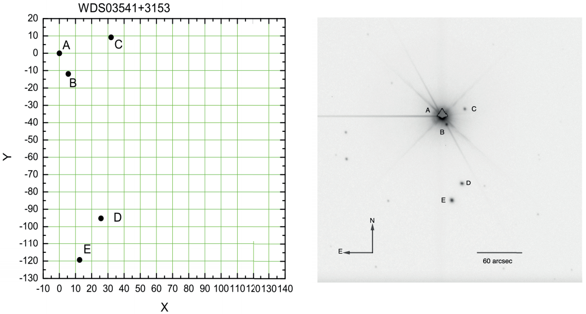
Fig. 9 The left image represents the components of the trapezium ADS 2843. The axes units are arcseconds. On the right, we show our observed image in the V filter, with N-E orientation and scale in arsecs. 3 seconds exposure time.
Table 20: Integration times for each filter for the trapezium ADS 2843
| Filter | Time (sec) |
|---|---|
| U | 10 |
| B | 5 |
| V | 3 |
| R | 2 |
| I | 1 |
We obtained 148 images for this trapezium in filters U - I, with exposure times of 0.2 and 0.5 seconds.
The right panel of Figure 9 shows the image of this trapezium in the V filter. Component A is clearly saturated, and its brightness affects component B making it impossible to obtain good photometric measurements.
In Table 21 we show the photometric radius for each component.
Table 21: Photometric aperture radii in pixels for trapezium ADS 2843
| r1 (pix) | r2 (pix) | r3 (pix) | |
|---|---|---|---|
| C | 8 | 10 | 12 |
| D | 12 | 14 | 16 |
| E | 12 | 14 | 16 |
In a similar manner as before, we use the transformation coefficients in Tables 1-5 and equations 1-5 to transform the number of counts for each star to intrinsic magnitudes and colours (see Table 22).
Table 22: Observed magnitudes and colours for ADS 2843
| U | B | V | R | I | U - B | B - V | V - R | R - I | V - I | |
|---|---|---|---|---|---|---|---|---|---|---|
| C | 12.79 | 12.39 | 11.44 | 11.00 | 10.69 | 0.40 | 0.95 | 0.44 | 0.31 | 0.75 |
| D | 11.49 | 11.07 | 10.22 | 9.87 | 9.67 | 0.41 | 0.85 | 0.35 | 0.20 | 0.55 |
| E | 10.62 | 10.27 | 9.79 | 9.66 | 9.61 | 0.35 | 0.48 | 0.13 | 0.05 | 0.18 |
Table 23 shows the spectral type associated to each star based on the value of its Q parameter.
Figure 10 shows the two-colour diagram for ADS 2843, where the red dots represent component C, D and E.
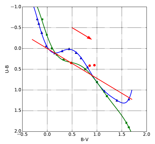
Figure 10: Two-colour diagram (U - B vs B - V) for ADS 2843. The colour figure can be viewed online.
From the two-colour diagram we obtain the values for the intrinsic colours, excesses, absorption and distance. However, in this case, the reddening lines for the components cross the intrinsic lines more than once. We have taken the excesses that appear to be more similar. Table 24 show the results for each case.
Table 24: Intrinsic colours, excesses, absorption and distances for ADS 2843
| Assuming Supergiant Stars | |||||||
|---|---|---|---|---|---|---|---|
| (U - B)0 | (B - V)0 | EU - B | EB - V | AV | Distance (pc) | Parallax (mas) | |
| C | -0.27 | 0.01 | 0.68 | 0.94 | 2.92 | 8989.06 | 0.11 |
| D | -0.17 | 0.04 | 0.58 | 0.81 | 2.51 | 6119.40 | 0.16 |
| E | 0.12 | 0.17 | 0.22 | 0.31 | 0.96 | 10113.19 | 0.10 |
| Assuming Main Sequence Stars | |||||||
| (U - B)0 | (B - V)0 | EU - B | EB - V | AV | Distance (pc) | Parallax (mas) | |
| C | -0.36 | -0.11 | 0.76 | 1.06 | 3.28 | 475.21 | 2.10 |
| D | -0.26 | -0.08 | 0.67 | 0.93 | 2.90 | 255.21 | 3.92 |
| E | 0.03 | 0.04 | 0.32 | 0.45 | 1.38 | 251.98 | 3.97 |
The magnitudes of the stars listed in SIMBAD come from the following reference: Høg et-al.(2000). Table 25 shows the comparison of our results with SIMBAD (*).
Table 25: Comparison with SIMBAD (*) for ADS 2843
| Magnitude | |||
|---|---|---|---|
| C | D | E | |
| U | 12.79 | 11.49 | 10.62 |
| U* | - | - | - |
| B | 12.39 | 11.07 | 10.27 |
| B* | - | 11.05 | 10.21 |
| V | 11.44 | 10.22 | 9.79 |
| V * | 11.24 | 10.36 | 9.92 |
| R | 11.00 | 9.87 | 9.66 |
| R * | - | 10.21 | - |
| I | 10.69 | 9.67 | 9.61 |
| I * | - | - | - |
| Spectral Type | |||
| C | D | E | |
| St | B8 | B9 | A0 |
| St* | - | - | A2V |
| Parallax | |||
| C | D | E | |
| Psg | 0.11 | 0.16 | 0.10 |
| Psp | 2.10 | 3.92 | 3.97 |
| P | 3.4918 | 7.3793 | 3.5114 |
We show the magnitudes dereddened with van de Hulst curve 15 in Table 26. This table assumes respectively supergiant stars and main sequence stars.
Table 26: Dereddened magnitudes and colour with van de Hulst curve 15 for ADS 2843
| Assuming Supergiant Stars | ||||||||||
|---|---|---|---|---|---|---|---|---|---|---|
| U | B | V | R | I | U - B | B - V | V - R | R - I | V - I | |
| C | 8.27 | 8.53 | 8.52 | 8.84 | 9.3 | -0.26 | 0.01 | -0.31 | -0.46 | -0.78 |
| D | 7.59 | 7.75 | 7.71 | 8 | 8.47 | -0.16 | 0.04 | -0.29 | -0.46 | -0.76 |
| E | 9.12 | 8.99 | 8.82 | 8.94 | 9.15 | 0.13 | 0.17 | -0.12 | -0.21 | -0.33 |
| Assuming Main Sequence Stars | ||||||||||
| U | B | V | R | I | U - B | B - V | V - R | R - I | V - I | |
| C | 7.7 | 8.04 | 8.15 | 8.56 | 9.12 | -0.35 | -0.11 | -0.41 | -0.56 | -0.97 |
| D | 6.99 | 7.24 | 7.32 | 7.72 | 8.28 | -0.25 | -0.08 | -0.39 | -0.57 | -0.96 |
| E | 8.48 | 8.44 | 8.41 | 8.63 | 8.95 | 0.03 | 0.04 | -0.22 | -0.32 | -0.54 |
2.2.4 ADS 16795
Trapezium ADS 16795 (also known as WDS 23300+5833) is located at RA=23h 30m, Dec=+58° 32 and has six components: AB, C, E, F, G and I, whose location is shown in Figure 11.
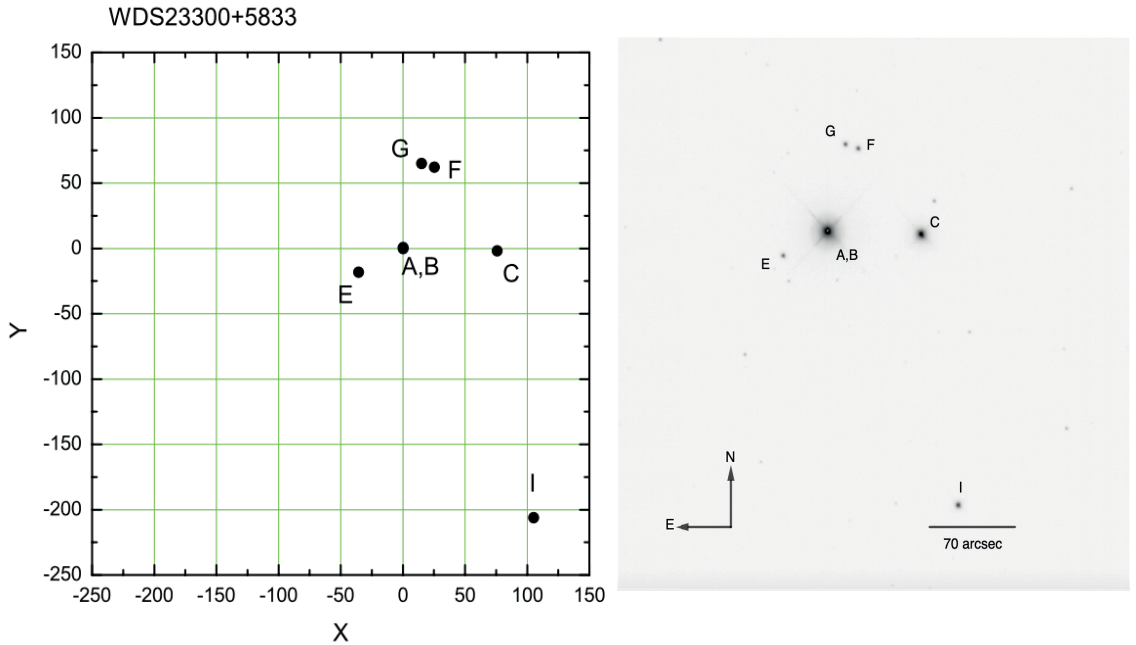
Fig. 11 The left image represents the components of the trapezium ADS 16795. The axes units are arcseconds. On the right, we show our observed image in the V filter, with N-E orientation and scale in arcsec. Exposure time is 5 seconds.
For this trapezium we obtained 144 images in filters U - I. This trapezium was observed on the night 2019, 14-15 December. For this night the transformation coefficients A, K and C for the filter U have no physical meaning (see Table 1), so no calculation of the U magnitude was possible.
Figure 11 shows the image of this trapezium in the V filter.
It is clear that the component AB is saturated so that the photometric measurements will only be performed on the other components (C, E, F, G and I).
Table 27 shows the photometric aperture radii for each component.
Table 27: Photometric Aperture radii for ADS 16795
| r1 (pix) | r2 (pix) | r3 (pix) | |
|---|---|---|---|
| C | 14 | 16 | 20 |
| E | 10 | 12 | 14 |
| F | 9 | 11 | 13 |
| G | 9 | 11 | 13 |
| I | 11 | 13 | 15 |
Table 28 gives the observed magnitudes and colours for the components of this trapezium. We obtained only those for the filters B, V, R and I because the results for U have no physical meaning and have been omitted.
Table 28: Observed magnitudes and colours for ADS 16795
| B | V | R | I | U - B | V - R | R - I | V - I | |
|---|---|---|---|---|---|---|---|---|
| C | 7.81 | 7.79 | 8.45 | 8.26 | 0.01 | 0.18 | -0.65 | -0.47 |
| E | 11.83 | 11.18 | 10.74 | 10.34 | 0.65 | 0.40 | 0.44 | 0.84 |
| F | 11.52 | 10.98 | 10.59 | 10.32 | 0.54 | 0.27 | 0.38 | 0.65 |
| G | 11.64 | 11.08 | 10.68 | 10.40 | 0.56 | 0.28 | 0.40 | 0.67 |
| I | 10.19 | 9.74 | 9.41 | 9.20 | 0.45 | 0.22 | 0.33 | 0.55 |
Since we cannot obtain a value of U, it is impossible to calculate the value of the Q parameter. The magnitudes of the stars listed in SIMBAD come from the following reference: Zacharias et-al.(2012). In Table 29 we compare our results with those listed in SIMBAD.
3 The slope of the reddening line
Since the Q-derived spectral types differ slightly from those listed in SIMBAD, we speculate that these differences might be due to slight differences in the value of the slope of the reddening line on the two-colour diagram from the canonical value(0.72).
The slope of the reddening line corresponds to the ratio of the colour excesses E(U - B) and E(B - V), and its value is clearly dependent on the physical and chemical properties of the interstellar medium through which the light from the stars travels on its way to our observing instruments. Carrying out a full investigation as to whether the slope of the reddening line differs from region to region is not only a rather interesting endeavour, but one that is clearly outside the scope of this paper. Here we shall only speculate that this might be the reason for the slight differences in stellar spectral types, and use the seven points we have to obtain a value for the new slope. [Aidelman Cidale(2023)] suggest that the possible difference of the slope of the reddening line from the canonical value may be due to an anomalous colour excess or to variations of the extinction law.
In Table 30 we present the object name, the Q-derived spectral type, the measured Q index, the SIMBAD spectral type and the value of the Q index for the spectral type given in Column 4.
Table 30: Q parameter values associated with the spectral value derived and the types given in the literature
| Object | STobs | Qobs | ST int | Qint |
|---|---|---|---|---|
| ADS15184C | B5 | -0.48 | B1.5 | -0.74 |
| ADS15184D | B6 | -0.40 | B1 | -0.78 |
| ADS4728C | B8 | -0.20 | B9 | -0.13 |
| ADS4728D | B3 | -0.63 | B1 | -0.78 |
| ADS4728E | B5 | -0.42 | B3 | -0.57 |
| ADS4728F | B9 | -0.08 | B9 | -0.13 |
| ADS4728I | B8 | -0.26 | B5 | -0.44 |
Figure 12 shows the relation we obtain from Table 31 between the observed Q index (Q obs ) and the Q associated to the spectral type reported in SIMBAD (Q int ). We fitted a least squares straight line that produced the following equation:
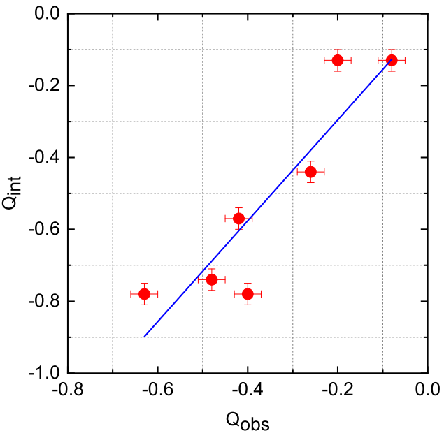
Table 31: Data for stars with discrepant Spectral types between the Q-derived value and the value found in SIMBAD
| Object | Spectral Type | (U - B)int | (B - V)Obs | (B - V)int | E(B - V) |
|---|---|---|---|---|---|
| ADS15184C | B1.5V | -0.88 | 0.32 | -0.25 | 0.57 |
| ADS15184D | B61V | -0.95 | 0.25 | -0.26 | 0.51 |
| ADS4728C | B9V | -0.18 | 0.21 | -0.07 | 0.28 |
| ADS4728D | B1V | -0.95 | 0.01 | -0.26 | 0.27 |
| ADS4728E | B3V | -0.68 | 0.10 | -0.20 | 0.30 |
| ADS4728F | B9V | -0.18 | 0.21 | -0.07 | 0.28 |
| ADS4728I | B8 | -0.36 | 0.12 | -0.11 | 0.23 |
Using this equation we might be able to correct the Q-derived spectral types. However, the number of points which produce this equation is very small so, at present, we have decided to leave its use and confirmation of usefulness for further investigations.
Algebraic manipulation of equation (7) allows us to express it as follows:
where m represents the possible new slope of the reddening line, and the suffixes int and Obs refer to the intrinsic and observed values. Effecting a least squares solution for m from this equation would allow us to explain the difference between the Q-derived spectral types and the spectral types listed in SIMBAD as a difference (from 0.72) of the slope of the reddening line on the two-colour diagram.
In what follows we shall use the information we have for the seven discrepant points and calculate a value for the slope of the reddening line that fits these results. In Table 31 we see in Column 1 the name of the star, in Column 2 the spectral type, in Column 3 the (U - B) int , in Column 4 (B - V) Obs , in Column 5 (B - V) int and in Column 6 E(B - V) for the stars for which a discrepant Q-derived spectral type was found.
Effecting a least squares solution for m in equation (8) using the values listed in Table (32) produces a value for the slope of the reddening line
4 Conclusions
This paper constitutes a photometric study of some trapezia in the Galaxy. The data were obtained during several observing seasons.
Here we present CCD photometry of the brighter stars in the stellar trapezia ADS 15184, ADS 4728, ADS 2843, and ADS 16795, which we have used to explore the possibility of finding the spectral type of the stars using the Q parameter, defined as Q = (U - B) - 0.72(B - V). This parameter is reddening independent, since the slope of the reddening line on the two-colour diagram is approximately equal to 0.72 (see Johnson & Morgan 1953). This, of course, is a first approach since the calibration we used for the Q parameter versus the spectral type does not take into consideration peculiar stars and is only based on typical stars of luminosity classes I and V.
The spectral types which we have determined coincide reasonably well with those listed in SIMBAD. However, a different value of the slope of the reddening line on the two-colour diagram might produce a better coincidence between the Q-derived spectral types and those listed in SIMBAD. Effecting a least squares solution for the slope of the reddening line in equation (8) produces a value of its slope m of
As part of our study we intend to determine the spectral type of the stars in the trapezia through classification of their spectra and hope to be able to measure their radial velocities which, joined with proper motions from GAIA will allow us to perform a detailed dynamical study of the Galactic trapezia.

