


 nueva página del texto (beta)
 Inglés (pdf)
 Artículo en XML
 Referencias del artículo
 Enviar artículo por email
 Citado por SciELO
  Similares en
SciELO
Similares en
SciELO 
 Permalink
1 Introduction
Galaxies are not uniformly distributed in the Universe, instead they undergo gravitational clustering that leads to an intricate three-dimensional structure in the shape of a network of knots, filaments, walls and voids (Libeskind et al. 2018). This cosmic web, revealed in both the observed distribution of galaxies (Geller & Huchra 1989; Santiago-Bautista et al. 2020) and in cosmological simulations (Davis et al. 1985; Springel et al. 2005), is called the Large-Scale Structure of the Universe (LSS, Peebles 1980; Einasto 2010), and contains systems of galaxies at different scales embedded in it (Einasto et al. 1984; Cautun et al. 2014). Such systems go from small groups, like the Local Group that hosts the Milky Way, to superclusters, the largest and youngest coherent structures formed under gravitational influence in the Universe (reaching up to ≈ 100 Mpc long, e.g., Oort 1983; Böhringer & Chon 2021).
Knot-shaped regions, that is, quasi-spherical overdensities of galaxies with radii ranging from
The baryonic -stellar and gaseous- matter contained in galaxies and in the form of intracluster X-ray emitting hot gas (intracluster medium, ICM, e.g., Böhringer & Werner 2010) is estimated (White 1992; Lima-Neto et al. 2005) to account for only 15% of the total mass of a galaxy system, while the remaining 85% is provided by the dark matter (DM). Nevertheless, as a first approximation, one can consider a group/cluster as a collisionless ensemble of galaxies moving in the mean gravitational field generated by its total mass (e.g., Schneider 2015). In this context, galaxies may be taken as fundamental observational tracers (or primary units, e.g., Padmanabhan 1993) of the global dynamical properties of the galaxy system.
The process of formation and evolution of a cluster from a matter density perturbation to a galaxy system in dynamical equilibrium is driven both by the initial cosmological conditions and by various physical and stochastic mechanisms (Binney & Tremaine 2008). Initially, both the homogeneous background and the matter perturbation expand with the Hubble flow; however, a fraction of this matter condenses into a set of galaxies that decouple from the expansion. The cluster itself, in the course of time, decouples from the expansion, forming now a gravitationally bound system, which turns around and begins a process of collapse that ends in an eventual virialization (Gunn & Gott III 1972). This is a state of statistical equilibrium of internal gravitational forces, reflected in the averages of the total kinetic and potential energies of galaxies (Limber & Mathews 1960). Analyzing the transitory evolutionary state of galaxy systems is not a trivial task, even when gravity is the sole driving force shaping their evolutionary processes. Here, we use the term ‘evolutionary state’ to refer to the degree of progress a galaxy system has in its evolutionary line, starting from its formation and ending at equilibrium (relaxation).
In this work we present a method to characterize the evolutionary state of galaxy systems by estimating the entropy component that depends only on the macroscopic state of their galaxy ensembles. For this, we propose a specific entropy estimator (H Z ) that combines (optical) observational parameters of the systems such as virial mass, volume, and galaxy velocity dispersion. Our fundamental premise is that a galaxy ensemble should evolve in the sense of increasing entropy, modifying its distribution of galaxies in the observed phase-space (which includes radial, angular and velocity coordinates) to a more random and dynamically relaxed one where there are no macroscopic movements or special configurations (Landau & Lifshitz 1980; Saslaw & Hamilton 1984). This means that the spatial and velocity distributions of member galaxies change as the system evolves, starting from more substructured ensembles (with less entropy) towards more homogeneous ones in dynamical relaxation (with higher entropy). Of course, the parameters associated with the global dynamics of the system also change in the process, and may be useful for the estimation of state functions such as entropy. No assumption is made here about the distribution of DM and ICM within the cluster ( Lokas & Mamon 2003; Lima-Neto et al. 2005), but only about their important contribution to the total gravitational potential that determines the dynamics of the galaxy ensemble.
To evaluate the H
Z
-entropy estimator we make use of different tests. The first is the comparison between H
Z
-entropy estimator and a discrete classification of assembling states applied to an observational samples of 70 nearby clusters (
In § 2, we extend the discussion about the dynamical equilibrium and stability of galaxy clusters, together with a brief description of the way evolutionary state is commonly characterized from observed and simulated data. In § 3, we focus on the entropy-based estimator and present our proposal to quantify the dynamical state of galaxy systems. In § 4, we apply our method to a sample of 70 well-sampled galaxy clusters in the nearby Universe, from very rich to poor ones. In § 5 we calculate the Shannon entropy for both the observational sample and a sample of 248 cluster halos from the IllustrisTNG simulation. Then, we compare this parameter with H
Z
. Other dynamical parameters are evaluated in § 6 also for validating H
Z
. Discussion and conclusions are presented in § 7. Throughout this paper we assume a flat
2 Evolution, equilibrium and stability of galaxy clusters
2.1 Reaching Virial Equilibrium
The evolution of galaxy systems at various scales is understood today through the hierarchical formation model (Peebles 1980; Padmanabhan 1993; Zakhozhay 2018) in a
Galaxy clustering is an irreversible process where, as galaxies accumulate, different mechanisms tend to increase the number of ways in which, in a statistical sense, internal energy can be distributed within the systems (Saslaw 1980; Saslaw & Hamilton 1984). Once bound and during collapse, the galaxy system undergoes internal -dissipationless- processes (e.g., violent relaxation, phase mixing, energy equipartition, galaxy mergers, fading of substructures and density or temperature gradients, among others, see, White 1996; Dehnen 2005; Binney & Tremaine 2008) that lead to states of greater dynamical relaxation. All these processes are dominated by gravitational interactions that, during the relaxation time, tend to homogenize the spatial distribution of the member galaxies and to distribute their radial velocities in a Gaussian way -inside the clusters, galaxies are scattered randomly (achieving a quasi-Maxwellian velocity distributions as they tend to virialization, e.g., Saslaw & Hamilton 1984; Sampaio & Ribeiro 2014), causing the tendency for macroscopic motions to disappear. This requires the individualization of the motions of the galaxies, so that any substructure (e.g., accreted groups) will be ‘dissolved’ before the cluster virializes. The thermodynamic perturbations and the changes in the distribution of the ICM inside the clusters during their evolution also produce increases in the total entropy of these systems (Tozzi & Norman 2001; Voit 2005).
The equilibrium state can be understood, in a first approximation, as that in which the gravitational collapse is supported by the effect of inertial -centrifugal or dispersion- forces, achieving relaxed internal configurations (called states of dynamical relaxation), that is, in which there are no unbalanced potentials, such as gravitational-driving forces, within galaxy systems. In this sense, collisionless systems in equilibrium are analogous to self-gravitating fluids because they support gravitational collapse through “pressure gradients” proportional to the velocity dispersion that, at each point, tend to disperse any local increase in particle density (Binney & Tremaine 2008). Furthermore, dynamical equilibrium is characterized by the statistical equality of the cluster mass profiles obtained from different galaxy populations within the cluster (Lokas & Mamon 2003; Lima-Neto et al. 2005), implying that all these populations are in equilibrium with the cluster potential according to the hydrodynamical equilibrium model by Jeans.
Throughout the evolution of an isolated cluster, its total internal energy U = K + W is conserved so that, as the member galaxies get closer together (spontaneous reduction of inter-particle distance r ij by mutual attraction), the gravitational potential energy W decreases (becoming more negative) and consequently the total internal kinetic energy K increases. This is reflected observationally as an increase in the velocity dispersion of galaxies, which can stop the collapse. Thus, when the system finds some route to dynamical equilibrium, the increase in K at the expense of the decrease in W does not continue indefinitely, but evolves toward configurations in which the ratio
tends to one (
a state in which dynamical parameters that characterize the global configuration of the system remain, at least temporarily, stationary (relaxed). The virial theorem expresses a statistical equilibrium between the temporal averages of the total internal kinetic and gravitational potential energies, i.e.,
2.2 Stability
Going beyond the description of equilibrium in galaxy systems, we need to discuss if this equilibrium is stable and this topic requires involving the concept of ‘entropy’. As any thermodynamic system, self-gravitating systems progress in the sense of increasing entropy (Lifshitz & Pitaevskii 1981; Tremaine, H´enon & Lynden-Bell 1986; Pontzen & Governato 2013) towards the state of dynamical equilibrium described above. Galaxy clustering simulations also confirm this fact (Saslaw & Hamilton 1984; Iqbal et al. 2006, 2011). Due to the scattering experienced by galaxies in the phase-space of clusters, these become the regions within the LSS where first-order entropy production occurs by increasing the randomness of the motion of galaxies during their gravitational accumulation. Even if galaxy clusters are isolated, some entropy is generated -or produced- due to the presence of internal irreversibilities. The peculiarity here is that the virial equilibrium is not unique, but only a metastable equilibrium state (Antonov 1962; Lynden-Bell & Wood 1968; Padmanabhan 1990; Chavanis et al. 2002). This means that the entropy of self-gravitating systems can grow indefinitely without reaching a global maximum, that is, the virial equilibrium is only a state of local extreme of entropy (Padmanabhan 1989).
The dynamical equilibrium of a galaxy cluster can be disturbed if it actively interacts with its surroundings, for example through mergers with other clusters and/or group accretions or tidal forces. As a result, the cluster takes a route towards a new equilibrium, in a state of higher entropy. Concerning the impact of the interaction, if the accreted groups are very small, the clusters can be kept unperturbed in states close to equilibrium. In more extreme cases, the merger of two massive clusters completely removes the systems from their equilibrium. In dense environments, such as supercluster cores, the accretion of galaxies and groups by the most massive clusters continually disturbs their dynamical states. On the other hand, in less dense environments, such as along filaments or edges near voids, clumpy clusters evolve as quasi-isolated systems, reaching dynamical relaxation possibly faster, without many significant disturbances, but accessing lower entropy levels compared to clusters in “busy” environments. That is, depending on the cosmological environment inside the LSS in which a cluster evolves, its relaxation process may be affected several times -or not- given the amount of matter available in its surroundings.
The most stable states of a galaxy cluster -of mass
2.3 Estimating the Evolutionary State of Galaxy Systems
Observationally, a cluster close to dynamical equilibrium is distinguished from a non-relaxed one by exhibiting a more regular morphology (Sarazin 1988), both in the optical and X-rays, and a more homogeneous -projected- spatial distribution of member galaxies (without the presence of significant substructures, Caretta et al. 2023, and references therein), as well as by having a more isotropic galaxy velocity distribution (or Gaussian in the line-of-sight, Girardi & Mezzetti 2001; Sampaio & Ribeiro 2014).
Concerning global morphology, the most dynamically relaxed clusters tend to present low ellipticity shapes in the projected distribution of galaxies and X-ray surface brightness maps, with a -possible- single peak at their centers. Several morphological classifications have been proposed following this premise (Sarazin 1988, and references therein). There are also indicators of the internal structure of the galaxy systems, such as the radial profile and the degree of concentration of galaxies (Adami et al. 1998; Tully 2015; Kashibadze et al. 2020), as well as a measure of the presence of substructures within them using 1D, 2D and 3D tests (Geller & Beers 1982; Dressler & Shectman 1988; Caretta et al. 2023).
In this sense, a significantly substructured system, either from optical observation of galaxy subclumps (e.g., Geller & Beers 1982; Bravo-Alfaro et al. 2009; Caretta et al. 2023) or the detection of multiple peaks in X-ray emission (e.g., Jones & Forman 1984; Buote & Tsai 1995; Lagan´a et al 2019), cannot be considered in dynamical equilibrium. Thus, the presence and significance of substructures reveal how far the galaxy system is from a relaxed and homogeneous global potential. A description of the cluster level of internal substructuring is called its gravitational assembly state (Caretta et al. 2023).
In principle, one can also measure global parameters related to the internal dynamics (Carlberg et al. 1996; Girardi & Mezzetti 2001) -or dynamical state- of the galaxy system. These parameters are associated, for example, with the mass, radius and velocity dispersion of the system. Such approach supposes that both the observable aspect and structure and the dynamical parameters of the system change in a correlated manner during its evolution, dominated by mechanisms that take it from more irregular and substructured configurations to those with more homogeneous galaxy distributions and more dynamically relaxed (Araya-Melo et al. 2009).
Furthermore, from X-ray observations one can construct entropy (or temperature or density) profiles that account for the evolutionary history, structure and thermodynamic state of the ICM inside the clusters (Tozzi & Norman 2001; Voit 2005), which also contributes to the study of the degree of relaxation -or disturbance- of their gravitational potentials (analysis of self-similarity of clusters). Nevertheless, we are not always fortunate enough to detect X-ray emission from clusters nor to have the amount of data necessary to carry out massive studies, so for this we are still limited to optical surveys.
3 Entropy of galaxy systems from global parameters
Based on the ‘classical’ concept of entropy of a particle system, it is possible to construct an estimator for the entropy component related to the set of member galaxies of a cluster, the ‘galaxy ensemble’. The depth of the cluster’s global potential well, which determines how fast the bound galaxies must move, is proportional to the total mass of the cluster that can be estimated, with negligible bias (see, Biviano et al. 2006), by the virial mass estimator
where
is the projected mean radius of the distribution of cluster galaxies, where
Now, as a first approximation, we can imagine the set of cluster galaxies as a system of particles with mean kinetic energy (Schneider 2015)
and confined in a region of volume
We assume that the velocity dispersion of galaxies is proportional to the ‘temperature’ T of the galaxy ensemble1, so that
matching the definition of the so-called gravitational pressure (Padmanabhan 2000), P = W/3V, when
In virial equilibrium, the internal energy of the galaxy ensemble is U = K + W = - K, according to (2). However, for any state of the system including those prior to equilibrium, the internal energy can be generalized, as in [ Hamilton 1984], in the form U = K(1 - 2b), where, for unbound systems (b = 0) the internal energy is only kinetic, while for bound and virialized systems (
where
As can be inferred from (3), galaxy systems of fixed mass internally heat up (T increases) when they contract (R
vir decreases) and cool down (T decreases) when they expand (R
vir increases). In addition, from (8) it is possible to appreciate an atypical behavior of virialized self-gravitating systems. If we allow the galaxy systems to exchange energy -but not matter- with the environment, then they cool down (
A fundamental expression of the form
It is necessary to use an expression analogous to the Gibbs Tds equation, but which conforms to the thermodynamic behavior of self-gravitating systems described above. In the considered galaxy ensemble the entropy increases along with the internal kinetic energy as they virialize (see, § 2). Then, we can impose that, in systems of point galaxies,
where, by analogy with the well-known thermodynamic expressions for temperature and pressure in the Gibbs Tds equation, we have
Note that, for self-gravitating galaxy systems in general, we need the
Finally, in order to obtain an estimator for the entropy of galaxy clusters, we will solve the system of differential equations (10) assuming that
where s
0 is an integration constant possibly related to the initial entropy of the galaxy ensemble, e.g., the entropy it had when the distribution of galaxies was not yet concentrated before gravitational clustering (see, § 2). Replacing the expressions
defined only in terms of observational parameters that can be obtained through optical data (e.g., galaxy coordinates and redshifts).
4 Testing the H Z entropy estimator in galaxy systems
4.1 Observational Data
We use data from [Caretta et al.2023], a sample of 67 galaxy clusters, from Abell/ACO (Abell 1958; Abell et al. 1989) catalogs, with redshifts up to
TABLE 1 Cluster sample (Top70)
| Optical data | X-ray datab | Basic properties | |||||||
|---|---|---|---|---|---|---|---|---|---|
| Namea | RACDG | DecCDG |
|
Na | r500 | kTx | σLOS |
|
Rvir |
| [deg] J2000 | [deg] J2000 | [Mpc] | [keV] | [km/s] | [1014 |
[Mpc] | |||
| (1) | (2) | (3) | (4) | (5) | (6) | (7) | (8) | (9) | (10) |
| A2798B | 9.37734 | -28.52947 | 0.1119 | 60 | 0.7476 | 3.39 | 757 | 6.01 | 1.75 |
| A2801 | 9.62877 | -29.08160 | 0.1122 | 35 | ... | 3.20 | 699 | 6.94 | 1.83 |
| A2804 | 9.90754 | -28.90620 | 0.1123 | 48 | ... | 1.00 | 516 | 3.11 | 1.40 |
| A0085A | 10.46052 | -9.30304 | 0.0553 | 318 | 1.2103 | 7.23 | 1034 | 19.75 | 2.65 |
| A2811B | 10.53718 | -28.53577 | 0.1078 | 103 | 1.0355 | 5.89 | 947 | 13.94 | 2.32 |
| A0118 | 13.75309 | -26.36238 | 0.1144 | 72 | ... | ... | 680 | 6.16 | 1.76 |
| A0119 | 14.06709 | -1.25549 | 0.0444 | 294 | 0.9413 | 5.82 | 853 | 9.51 | 2.08 |
| A0122 | 14.34534 | -26.28134 | 0.1136 | 28 | 0.8165 | 3.70 | 677 | 4.98 | 1.64 |
| A0133A | 15.67405 | -21.88215 | 0.0562 | 86 | 0.9379 | 4.25 | 778 | 7.30 | 1.90 |
| A2877-70 | 17.48166 | -45.93122 | 0.0238 | 112 | 0.6249 | 3.28 | 679 | 4.20 | 1.60 |
| AM0227-334 | 37.33891 | -33.53196 | 0.0780 | 30 | ... | ... | 625 | 4.11 | 1.56 |
| A3027A | 37.70601 | -33.10375 | 0.0784 | 82 | 0.7200 | 3.12 | 713 | 7.52 | 1.90 |
| A0400 | 44.42316 | 6.02700 | 0.0232 | 51 | 0.6505 | 2.25 | 343 | 0.68 | 0.87 |
| A0399 | 44.47120 | 13.03080 | 0.0705 | 69 | 1.1169 | 6.69 | 950 | 11.65 | 2.21 |
| A0401 | 44.74091 | 13.58287 | 0.0736 | 114 | 1.2421 | 7.06 | 1026 | 15.11 | 2.41 |
| A3094A | 47.85423 | -26.93122 | 0.0685 | 84 | 0.6907 | 3.15 | 637 | 4.83 | 1.65 |
| A3095 | 48.11077 | -27.14017 | 0.0652 | 21 | ... | ... | 327 | 0.65 | 0.84 |
| A3104 | 48.59055 | -45.42024 | 0.0723 | 28 | 0.8662 | 3.56 | 498 | 1.77 | 1.18 |
| S0334 | 49.08556 | -45.12110 | 0.0746 | 26 | ... | ... | 534 | 2.11 | 1.25 |
| S0336 | 49.45997 | -44.80069 | 0.0773 | 32 | ... | ... | 538 | 3.02 | 1.40 |
| A3112B | 49.49025 | -44.23821 | 0.0756 | 74 | 1.1288 | 5.49 | 705 | 8.45 | 1.98 |
| A0426A | 49.95098 | 41.51168 | 0.0176 | 314 | 1.2856 | 6.42 | 1029 | 13.50 | 2.36 |
| S0373 | 54.62118 | -35.45074 | 0.0049 | 98 | 0.4017 | 1.56 | 390 | 0.43 | 0.75 |
| A3158 | 55.72063 | -53.63130 | 0.0592 | 249 | 1.0667 | 5.42 | 1066 | 13.93 | 2.35 |
| A0496 | 68.40767 | -13.26196 | 0.0331 | 279 | 0.9974 | 4.64 | 712 | 6.31 | 1.82 |
| A0539 | 79.15555 | 6.44092 | 0.0288 | 92 | 0.7773 | 3.04 | 698 | 3.92 | 1.56 |
| A3391 | 96.58521 | -53.69330 | 0.0560 | 75 | 0.8978 | 5.89 | 817 | 7.74 | 1.94 |
| A3395 | 96.90105 | -54.44936 | 0.0496 | 199 | 0.9298 | 5.10 | 746 | 6.42 | 1.82 |
| A0576 | 110.37600 | 55.76158 | 0.0379 | 191 | 0.8291 | 4.27 | 866 | 11.18 | 2.20 |
| A0634 | 123.93686 | 58.32109 | 0.0268 | 70 | ... | ... | 395 | 1.13 | 1.03 |
| A0754 | 137.13495 | -9.62974 | 0.0542 | 333 | 1.1439 | 8.93 | 820 | 9.10 | 2.05 |
| A1060 | 159.17796 | -27.52858 | 0.0123 | 343 | 0.7015 | 2.79 | 678 | 3.99 | 1.57 |
| A1367 | 176.00905 | 19.94982 | 0.0215 | 226 | 0.9032 | 3.81 | 597 | 3.76 | 1.54 |
| A3526A | 192.20392 | -41.31167 | 0.0100 | 126 | 0.8260 | 3.40 | 564 | 2.43 | 1.34 |
| A3526B | 192.51645 | -41.38207 | 0.0155 | 45 | ... | ... | 317 | 0.44 | 0.75 |
| A3530 | 193.90001 | -30.34749 | 0.0536 | 94 | 0.8043 | 3.62 | 631 | 4.63 | 1.63 |
| A1644 | 194.29825 | -17.40958 | 0.0470 | 288 | 0.9944 | 5.25 | 1008 | 13.98 | 2.36 |
| A3532 | 194.34134 | -30.36348 | 0.0557 | 58 | 0.9201 | 4.63 | 443 | 1.66 | 1.16 |
| A1650 | 194.67290 | -1.76139 | 0.0842 | 146 | 1.1015 | 5.72 | 723 | 7.55 | 1.90 |
| A1651 | 194.84383 | -4.19612 | 0.0849 | 158 | 1.1252 | 7.47 | 876 | 12.48 | 2.25 |
| A1656 | 194.89879 | 27.95939 | 0.0233 | 919 | 1.1378 | 7.41 | 995 | 15.66 | 2.47 |
| A3556 | 201.02789 | -31.66996 | 0.0482 | 90 | ... | 3.08 | 520 | 2.59 | 1.35 |
| A1736A | 201.68378 | -27.43940 | 0.0350 | 36 | 0.9694 | 3.34 | 386 | 1.30 | 1.08 |
| A1736B | 201.86685 | -27.32468 | 0.0456 | 126 | ... | ... | 844 | 8.82 | 2.03 |
| A3558 | 201.98702 | -31.49547 | 0.0483 | 469 | 1.1010 | 5.83 | 955 | 15.75 | 2.46 |
| SC1329-313 | 202.86470 | -31.82058 | 0.0448 | 46 | ... | ... | 383 | 1.01 | 0.99 |
| A3562 | 203.39475 | -31.67227 | 0.0486 | 82 | 0.9265 | 5.10 | 594 | 3.94 | 1.55 |
| A1795 | 207.21880 | 26.59301 | 0.0630 | 154 | 1.2236 | 6.42 | 780 | 7.09 | 1.88 |
| A2029 | 227.73377 | 5.74491 | 0.0769 | 155 | 1.3344 | 8.45 | 931 | 7.82 | 1.93 |
| A2040B | 228.19782 | 7.43426 | 0.0451 | 104 | ... | 2.41 | 627 | 4.77 | 1.65 |
| A2052 | 229.18536 | 7.02167 | 0.0347 | 120 | 0.9465 | 2.88 | 648 | 4.28 | 1.60 |
| MKW03S | 230.46613 | 7.70888 | 0.0443 | 75 | ... | ... | 607 | 3.46 | 1.49 |
| A2065 | 230.62053 | 27.71228 | 0.0730 | 168 | 1.0480 | 6.59 | 1043 | 17.01 | 2.50 |
| A2063A | 230.77210 | 8.60918 | 0.0345 | 142 | 0.9020 | 3.34 | 762 | 6.18 | 1.81 |
| A2142 | 239.58345 | 27.23335 | 0.0902 | 157 | 1.3803 | 11.63 | 828 | 11.06 | 2.16 |
| A2147 | 240.57086 | 15.97451 | 0.0363 | 397 | 0.9351 | 4.26 | 935 | 15.70 | 2.47 |
| A2151 | 241.28754 | 17.72997 | 0.0364 | 276 | 0.7652 | 2.10 | 768 | 8.35 | 2.00 |
| A2152 | 241.37175 | 16.43579 | 0.0443 | 64 | 0.5783 | 2.41 | 406 | 1.56 | 1.14 |
| A2197 | 246.92114 | 40.92690 | 0.0304 | 185 | 0.5093 | 2.21 | 573 | 4.21 | 1.59 |
| A2199 | 247.15949 | 39.55138 | 0.0303 | 459 | 1.0040 | 4.04 | 779 | 7.21 | 1.91 |
| A2204A | 248.19540 | 5.57583 | 0.1518 | 38 | 1.3998 | 10.24 | 1101 | 20.33 | 2.59 |
| A2244 | 255.67697 | 34.06010 | 0.0993 | 102 | 1.1295 | 5.99 | 1161 | 18.35 | 2.55 |
| A2256 | 256.11353 | 78.64056 | 0.0586 | 280 | 1.1224 | 8.23 | 1222 | 20.63 | 2.68 |
| A2255 | 258.11981 | 64.06070 | 0.0805 | 179 | 1.0678 | 7.01 | 1000 | 16.44 | 2.47 |
| A3716 | 312.98715 | -52.62983 | 0.0451 | 123 | ... | 2.19 | 783 | 6.99 | 1.88 |
| S0906 | 313.18958 | -52.16440 | 0.0482 | 26 | ... | ... | 440 | 1.46 | 1.11 |
| A4012A | 352.96231 | -34.05553 | 0.0542 | 39 | ... | ... | 575 | 3.15 | 1.44 |
| A2634 | 354.62244 | 27.03130 | 0.0309 | 166 | 0.7458 | 3.71 | 717 | 5.87 | 1.78 |
| A4038A-49 | 356.93768 | -28.14071 | 0.0296 | 180 | 0.8863 | 2.84 | 753 | 5.95 | 1.79 |
| A2670 | 358.55713 | -10.41900 | 0.0760 | 251 | 0.9113 | 4.45 | 970 | 9.91 | 2.09 |
a A capital letter after the ACO name indicates the line-of-sight component of the cluster. b Taken from Caretta et al. (2023) and references therein.
By using different 1D, 2D and 3D methods (e. g., Dressler & Shectman 1988), applied to the distribution of the members inside the caustics, these authors searched for optical substructures in the cluster sample, supplementing their analysis with X-rays and radio literature data. They found that at least 70% of the clusters in their sample present clear signs of substructuring, with 57% being significantly substructured. The significance of the identified substructures in each cluster was estimated by the fraction of galaxies they contain with respect to the total richness.
The clusters were classified into five assembly state levels according to the presence -or not- and relative importance of substructures: unimodal systems, made up of a regular structure (U); low mass unimodal systems (L); systems with a primary structure and only low significance substructures (P); significantly substructured systems with one main substructure (S); and multimodal conglomerates with more than one main substructure (M). While the L clusters are young poor galaxy systems, representing evolutionary states prior to amalgamation processes but already relatively placidly evolved, the U clusters are old and massive, which have probably grown by mergers and accretions and have already settled close to a relaxation state. P clusters are also old and massive, but still present signs of recent accretions; since these accretions are minor, the relaxation state of the cluster is almost unaffected. Finally, S and M clusters are systems during merging processes, the difference being whether these mergers are minor or major, respectively.
The benefit of using this sample lies in the availability of this discrete classification of gravitational assembly states (see Column 2 of Table 2 below). This will serve to establish correlations between the H Z estimator applied to the ensemble of galaxies of each cluster and the evolutionary state obtained from direct observational methods.
TABLE 2 Dynamical parameters for Top70 cluster sample
| Name |
|
H Z | H S | r' c |
|
c K | c NFW | c 1MC |
|---|---|---|---|---|---|---|---|---|
| [nat] | [Mpc] | |||||||
| (1) | (2) | (3) | (4) | (5) | (6) | (7) | (8) | (9) |
| A2798B | U | 15.54 | 10.85 | 0.28 | 0.808 | 7.85 | 3.91 | 2.33 |
| A2801 | U | 15.34 | 10.60 | 0.29 | 0.794 | 3.94 | 1.22 | ... |
| A2804 | M | 14.58 | 10.16 | 0.22 | 0.668 | 3.41 | 1.55 | ... |
| A0085A | S | 16.26 | 12.48 | 0.42 | 0.816 | 4.76 | 1.89 | 2.18 |
| A2811B | S | 16.09 | 11.69 | 0.37 | 0.762 | 5.42 | 1.77 | 2.23 |
| A0118 | S | 15.27 | 11.25 | 0.28 | 0.680 | 1.76 | 1.17 | ... |
| A0119 | S | 15.77 | 11.90 | 0.33 | 0.893 | 7.00 | 3.88 | 2.21 |
| A0122 | U | 15.26 | 10.72 | 0.26 | 0.839 | 8.29 | 5.03 | 2.00 |
| A0133A | S | 15.55 | 11.26 | 0.30 | 0.792 | 7.10 | 3.36 | 2.02 |
| A2877-70 | S | 15.18 | 10.99 | 0.25 | 0.828 | 10.59 | 6.95 | 2.55 |
| AM0227-334 | L | 15.03 | 9.36 | 0.25 | 0.650 | 3.72 | 1.97 | ... |
| A3027A | S | 15.36 | 11.20 | 0.30 | 0.825 | 3.32 | 1.26 | 2.64 |
| A0400 | S | 13.47 | 8.65 | 0.14 | 0.816 | 7.32 | 3.46 | 1.33 |
| A0399 | U | 16.07 | 12.03 | 0.35 | 0.775 | 6.43 | 4.61 | 1.97 |
| A0401 | U | 16.26 | 12.25 | 0.38 | 0.841 | 8.86 | 5.43 | 1.93 |
| A3094A | U | 15.06 | 11.13 | 0.26 | 0.865 | 3.93 | 1.28 | 2.38 |
| A3095 | L | 13.39 | 7.66 | 0.13 | 0.645 | 1.95 | 0.56 | ... |
| A3104 | S | 14.45 | 9.54 | 0.19 | 0.704 | 7.52 | 4.44 | 1.35 |
| S0334 | L | 14.63 | 9.77 | 0.20 | 0.757 | 12.41 | 7.42 | ... |
| S0336 | L | 14.65 | 9.39 | 0.22 | 0.730 | 4.84 | 1.38 | ... |
| A3112B | S | 15.33 | 11.11 | 0.32 | 0.756 | 1.98 | 1.32 | 1.75 |
| A0426A | P | 16.22 | 12.48 | 0.38 | 0.824 | 11.44 | 7.29 | 1.83 |
| S0373 | S | 13.78 | 9.13 | 0.12 | 0.823 | 6.11 | 2.58 | 1.86 |
| A3158 | S | 16.34 | 12.28 | 0.37 | 0.761 | 10.73 | 8.35 | 2.20 |
| A0496 | S | 15.31 | 11.54 | 0.29 | 0.919 | 6.26 | 2.99 | 1.82 |
| A0539 | S | 15.26 | 10.91 | 0.25 | 0.814 | 10.51 | 5.45 | 2.00 |
| A3391 | U | 15.67 | 11.38 | 0.31 | 0.804 | 9.75 | 5.43 | 2.15 |
| A3395 | M | 15.44 | 11.50 | 0.29 | 0.781 | 6.67 | 3.64 | 1.96 |
| A0576 | S | 15.80 | 11.98 | 0.35 | 0.830 | 6.26 | 2.93 | 2.65 |
| A0634 | L | 13.83 | 9.31 | 0.16 | 0.746 | 2.41 | 0.68 | ... |
| A0754 | M | 15.68 | 12.07 | 0.33 | 0.836 | 4.88 | 2.04 | 1.78 |
| A1060 | P | 15.17 | 11.29 | 0.25 | 0.874 | 9.76 | 6.62 | 2.24 |
| A1367 | M | 14.86 | 10.64 | 0.24 | 0.848 | 4.10 | 1.61 | 1.70 |
| A3526A | P | 14.71 | 10.33 | 0.21 | 0.823 | 8.40 | 4.62 | 1.61 |
| A3526B | S | 13.27 | 7.57 | 0.12 | 0.725 | 4.26 | 1.16 | ... |
| A3530 | S | 15.03 | 11.07 | 0.26 | 0.888 | 5.42 | 2.24 | 2.02 |
| A1644 | P | 16.19 | 12.39 | 0.38 | 0.838 | 7.51 | 5.26 | 2.37 |
| A3532 | S | 14.14 | 9.75 | 0.18 | 0.778 | 3.59 | 1.19 | 1.26 |
| A1650 | U | 15.40 | 11.32 | 0.30 | 0.846 | 3.42 | 1.26 | 1.72 |
| A1651 | P | 15.88 | 11.97 | 0.36 | 0.833 | 4.42 | 1.67 | 1.99 |
| A1656 | S | 16.14 | 12.73 | 0.39 | 0.861 | 7.79 | 4.11 | 2.17 |
| A3556 | M | 14.54 | 10.85 | 0.21 | 0.744 | 3.79 | 1.49 | ... |
| A1736A | S | 13.78 | 9.34 | 0.17 | 0.783 | 2.75 | 0.71 | 1.10 |
| A1736B | S | 15.75 | 11.77 | 0.32 | 0.775 | 5.74 | 3.64 | ... |
| A3558 | P | 16.06 | 12.60 | 0.39 | 0.826 | 4.89 | 2.12 | 2.23 |
| SC1329-313 | L | 13.77 | 8.65 | 0.16 | 0.744 | 4.63 | 2.34 | ... |
| A3562 | U | 14.87 | 10.70 | 0.25 | 0.841 | 4.15 | 1.74 | 1.67 |
| A1795 | U | 15.56 | 11.51 | 0.30 | 0.893 | 9.47 | 5.04 | 1.53 |
| A2029 | U | 16.02 | 11.81 | 0.31 | 0.838 | 12.94 | 6.92 | 1.44 |
| A2040B | S | 15.00 | 10.76 | 0.26 | 0.838 | 4.28 | 1.10 | ... |
| A2052 | S | 15.08 | 10.98 | 0.25 | 0.850 | 6.82 | 3.69 | 1.69 |
| MKW03S | U | 14.92 | 11.30 | 0.24 | 0.881 | 6.58 | 4.01 | ... |
| A2065 | U | 16.30 | 12.19 | 0.40 | 0.882 | 9.11 | 5.24 | 2.38 |
| A2063A | P | 15.48 | 11.50 | 0.29 | 0.899 | 9.51 | 5.19 | 2.00 |
| A2142 | P | 15.74 | 12.12 | 0.34 | 0.866 | 4.54 | 1.82 | 1.56 |
| A2147 | M | 15.99 | 12.00 | 0.39 | 0.829 | 3.62 | 1.64 | 2.63 |
| A2151 | M | 15.50 | 11.85 | 0.32 | 0.823 | 4.18 | 1.36 | 2.61 |
| A2152 | M | 13.91 | 9.38 | 0.18 | 0.758 | 1.99 | 0.75 | 1.96 |
| A2197 | M | 14.76 | 10.65 | 0.25 | 0.699 | 1.59 | 1.06 | 3.12 |
| A2199 | P | 15.53 | 12.02 | 0.30 | 0.884 | 7.41 | 4.23 | 1.89 |
| A2204A | S | 16.51 | 11.16 | 0.41 | 0.769 | 3.92 | 1.72 | 1.84 |
| A2244 | U | 16.60 | 12.33 | 0.41 | 0.821 | 10.46 | 7.81 | 2.25 |
| A2256 | S | 16.68 | 12.47 | 0.43 | 0.607 | 10.87 | 8.49 | 2.39 |
| A2255 | S | 16.20 | 12.31 | 0.39 | 0.789 | 6.54 | 3.42 | 2.31 |
| A3716 | M | 15.56 | 11.56 | 0.30 | 0.769 | 5.53 | 3.17 | ... |
| S0906 | L | 14.12 | 9.30 | 0.18 | 0.793 | 2.94 | 0.74 | ... |
| A4012A | L | 14.80 | 10.13 | 0.23 | 0.834 | 4.26 | 1.63 | ... |
| A2634 | S | 15.32 | 11.60 | 0.28 | 0.861 | 6.69 | 3.81 | 2.38 |
| A4038A-49 | S | 15.45 | 11.35 | 0.28 | 0.820 | 9.73 | 5.12 | 2.01 |
| A2670 | U | 16.12 | 11.92 | 0.33 | 0.859 | 10.24 | 6.01 | 2.29 |
a Gravitational assembly classes from Caretta et al. (2023).
The observational cluster sample is reported in Table 1: Column 1 shows the name of clusters; Columns 2, 3 and 4 present their right ascension, declination and mean redshift, respectively; Column 5 presents the number of presumably virialized sampled galaxies belonging to the system (inside the caustics and the aperture
For each observed cluster, the virial mass was estimated using (3) and the virial radius by
where
4.2 Simulation Data
In addition, we use data from the IllustrisTNG simulation (Springel et al. 2018; Nelson et al. 2019), a set of cosmological simulations that assumes initial conditions consistent with the [Collaboration 2016] results and takes into account magnetohydrodynamical effects. In particular, we use the TNG300-1 data cube that contemplates the largest volume allowing the study of the distribution of galaxies and massive objects such as clusters. We take halos (equivalent to galaxy clusters) from the TNG300-1 simulation at redshift z = 0,2 which has a resolution of 25003 dark matter particles and 25003 baryonic matter particles. We sampled 248 halos with masses greater than
Each halo in the simulation contains, on average, 1,300 subhalos within its virial radius, greatly outnumbering the tracers (galaxies) in our observational sample of clusters. This large difference is due to the number of low-mass systems (dwarf galaxies subhalos) entering the count of TNG300-1; these galaxies are hard to detect in real clusters due to their low luminosity. Thus, to avoid statistical differences between the parameters estimated from observational and simulated data, we limit the selection of member subhalos by taking only those with mass greater than
Figure 1 shows the projected distribution of member subhalos for two halos in the sample, one high-entropy (left) and one low-entropy (right). Note that, as expected, the distribution of subhalos is more random and homogeneous in a high entropy halo, while more substructured and elongated in a low entropy halo. This also happens in the observed clusters, reinforcing our hypothesis that evolutionary changes in galaxy systems progress in the direction in which the system dissolves substructures, becoming observationally more regular and homogeneous, with higher entropy values.
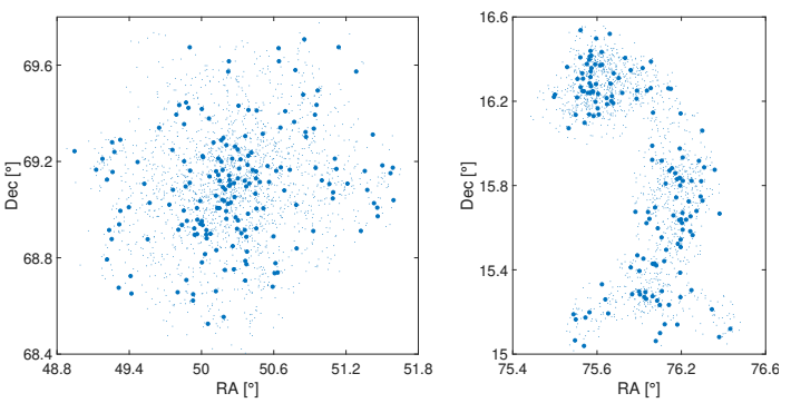
Fig. 1 Two examples of sampled TNG300 halos. Left: subhalo distribution for a high entropy halo (TNG-halo-34). Right: subhalo distribution for a low entropy halo (TNG-halo-87). Each dot represents a member subhalo: the small dots are subhalos with masses less than
4.3 Results on the Assembly State of Observed Clusters
To appreciate the correlation between the H Z entropy (shown in Column 3 of Table 2 below) and the gravitational assembly level -and therefore with the evolutionary state- of galaxy systems, we present in Figure 2 the distributions of the H Z values with respect to the assembly state classes. These are displayed in the form of boxplots, which allow graphically describing the locality, dispersion and asymmetry of data classes (groups) of a quantitative variable through its quartiles (Heumann & Shalabh 2016). The classes were ordered from more to less relaxed systems. Although the box overlap does not allow one to unambiguously discriminate the class to which an arbitrary individual cluster should belong, the statistical correlation is clear: the sequence U-P-S-M-L follows directly the decreasing median values of entropy. The only marginal difference case is between U and P systems, which is understandable if we consider that the primary systems (with only low significance substructures) are dynamically very similar to the unimodal ones -both tend to be relatively massive and evolved systems. This discussion will be resumed later.
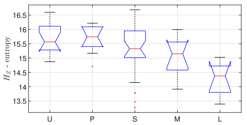
Fig. 2. Boxplots of H Z -entropy for the five assembly classifications of clusters. The lower and upper extremes of each box are the 25th and 75th percentiles, respectively, while the central red line marks the median. Whiskers extend to the most extreme non-outlier data, while outliers are represented by red ‘+’ symbols. The color figure can be viewed online.
5 Testing statistically the H Z -entropy estimator
5.1 Shannon Entropy of Galaxy Distributions in Phase-Spaces
Another way to evaluate the entropy estimates that H
Z
can provide is by using a method that does not take into account equilibrium assumptions, but allows us to characterize the internal states of a galaxy system from the raw distribution of its member galaxies. In information theory, for example, entropy is a measure of the uncertainty of a random variable (or source of information, e.g., Shannon 1948; Cover & Thomas 2006). If X is a discrete random variable with possible observable values
where the sum is performed over all possible values of the variable, and the base
Now, the raw coordinates of the galaxies in a cluster, i.e. the observable set of triples
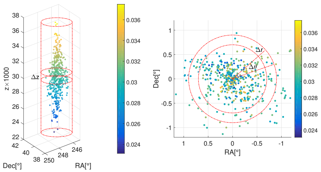
Fig. 3 Sample of galaxies for A2199 cluster in Caretta et al. (2023). Color bars represent the redshift (z) distribution. Left panel: the cylinder along the line-of-sight direction. Right panel: projected distribution in the sky plane with RA and Dec coordinates transported to the origin (the FRG, see the text). The color figure can be viewed online.
By considering the cylinder of sampled galaxies as a source of information for the x-distribution, the probability of finding a galaxy in the neighborhood of position x (i.e., the probability that the position random variable X takes a value very close to x inside the cylinder) can be approximated as
where
Shannon entropy is a well-established measure for quantifying disorder or uncertainty in a system (Cover & Thomas 2006). In this context, H S provides a measure of the degree of randomness in the distribution of galaxies in the phase-space of a cluster (or any other galaxy system). By calculating this entropy, we are evaluating the information contained in the galaxy ensemble and how galaxies are distributed in different regions of phase-space. Close to equilibrium, the memory (information) of the initial conditions of cluster formation is lost (Binney & Tremaine 2008; Araya-Melo et al. 2009). The general character of H S comes from the fact that it is not restricted only to thermodynamic variables, but to any type of data X that contains information about the state of a system, so it can be used to study characteristics of non-equilibrium systems as they evolve. In addition, it does not consider the microstates of a system as equiprobable, keeping a certain relationship in mathematical form and meaning with the Gibbs entropy (Jaynes 1957). .
5.2 Shannon Entropy Estimations
To calculate the Shannon entropy, we first established the observed joint PDF
On the other hand, as is evident in the right panel of Figure 3, galaxies with the highest and lowest redshifts prefer the center of the projected distribution of the cluster. This correlation between the variables r and z is physically justified since the galaxies acquire a greater speed during their transit through the central regions of the clusters (i.e., where the gravitational potential well is the deepest). Projection effects can also occur, especially for halo galaxies that are located in front or behind the core and close to the line-of-sight. No significant correlation was detected between the variables r or z with
Two statistical tests, Kolmogorov-Smirnov and Rank-Sum, showed no significant differences between both methods, confirming the null hypothesis that the PDFs
varying one of the variables in its respective domain (e.g.,
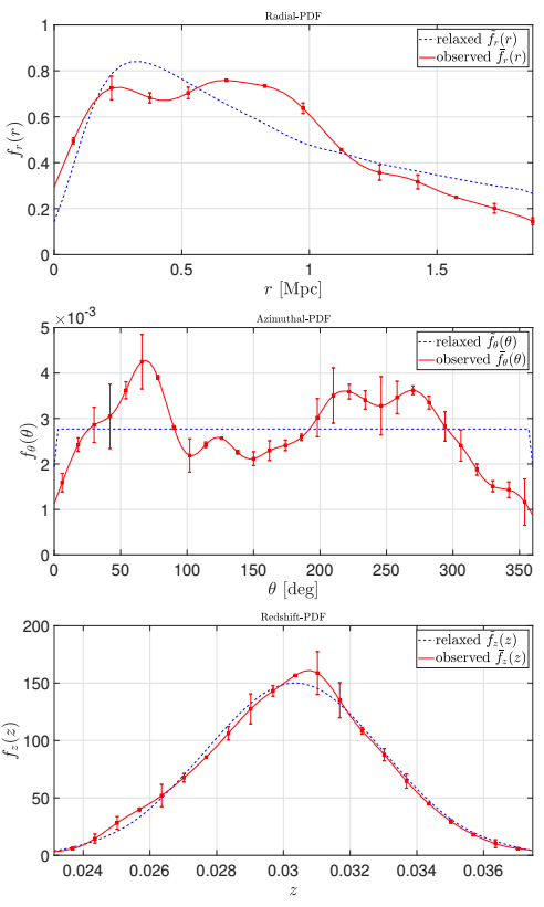
Fig. 4 Probability density functions for the radial-r, azimuthal-
5.3 Results on the Shannon Entropy for Observed and Simulated Clusters
The relation between the H Z -entropy estimator, proposed in the present work, and the Shannon entropy H S of the real galaxy distributions can be seen in Figure 5, where the dashed line represents the best fit curve, with a coefficient of determination (R 2, Heumann & Shalabh 2016) of 0.886. This figure shows a high degree of correlation (almost linear) between the H Z and H S entropies that, when measured by the Pearson and Spearman coefficients (e.g., Gibbons & Chakraborti 2003; Heumann & Shalabh 2016), gives the values 0.932 and 0.922, respectively. Below (see, §7), we offer what we believe to be a possible explanation for such an explicit correlation. In addition, the figure also shows the association of these H Z and H S entropy values with the assembly state of the clusters (represented by the U-P-S-M-L classes). Although the correlation is not evident, it is noticeable that all U and P clusters are placed in the locus of points with higher values of both H Z and H S , while all L are located in the region with lower values of these entropies.
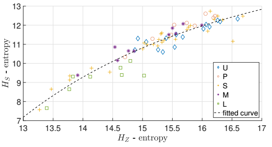
Fig. 5 Scatter plot of H
Z
vs. H
S
made with the entropy values estimated for the Top70 clusters. The symbols and color scale of the points represent the U-P-S-M-L assembly level classification of clusters performed by Caretta et al. (2023). The dashed line represents the best -power law- fit with
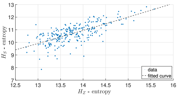
A procedure similar to that performed with Top70 clusters was applied to the TNG300 sample to compare the H Z and H S entropies estimated for the simulated halos. Figure 6 shows a significant correlation, with Pearson and Spearman coefficients of 0.709 and 0.678, respectively, between the dynamical and Shannon entropies, which are very similar to those of real clusters. We did not carry out a classification of simulated clusters in their different assembly levels (A) that allows us to analyze the distribution of H Z in each class, as in the case of real clusters. We hope to do this in future work.
6 Other validations for H Z
6.1 The Relaxation Probability of Galaxy Systems
Several studies reveal that clusters close to dynamical equilibrium have distributions of galaxies whose radial density and LOS velocity profiles tend to ones that can be represented by specific mathematical functions (Saslaw & Hamilton 1984; Sarazin 1988; Adami et al. 1998; Sampaio & Ribeiro 2014). The above is also true for the ICM entropy profiles in X-ray observations (e. g., Voit 2005) or for the distribution of DM subhalos in cosmological simulations (Davis et al. 1985; Springel et al. 2005). Thus, we consider that it is also possible to characterize the evolutionary state of a galaxy system by measuring how far the currently observed PDFs are from their expected equilibrium functional shapes. For this, we need to use (or choose) a consistent reference equilibrium model that describes the distribution when the galaxy ensemble is relaxed, as well as a metric that allows us to estimate the distance of the observed distribution from that of the equilibrium model.
We limit ourselves to a simple reference equilibrium model, considering clusters represented by a spherical distribution of galaxies, with a homogeneous core-halo spatial configuration and an isotropic velocity distribution without net angular momentum.
In principle, the radial distribution of galaxies can be well described [?, see]]ad1998 by different single mass profiles proposed for clusters in the literature, both core- (King 1962; Einasto 1965) and cuspy- (Hernquist 1990; Navarro, Frenk & White 1996) dominated ones. Nonetheless, there has been a tendency, especially for fitting DM halos, to use more complex functions, with a larger number of free parameters (Dehnen 1993; Fielder et al. 2020; Diemer 2023) -although they are essentially double and/or truncated power laws- in order to better accommodate the inner and outer slopes. On the other hand, since core-dominated profiles usually perform slightly better for real clusters (Sarazin 1988; Adami et al. 1998; García-Manzanárez 2022) -as commented before, the core-halo structure is the one expected for self-gravitating systems at equilibrium- and considering the simplest possible analytical form, we choose the King density profile at this point. Such a profile can be approximated analytically by the form
suggesting a finite central density
in which the count of galaxies must be performed in bins of length
For the azimuthal distribution of galaxies on the RA-Dec projected plane of a regular cluster we expect a continuous uniform azimuthal-PDF of the form
since, under the assumed equilibrium model, the probability of finding galaxies in any direction of the plane must be the same if there are no deformities (flattening or elongation) in the cluster morphology and no substructures when counting galaxies in slices of width
Finally, for the (3D) galaxy velocities inside clusters in equilibrium we expect a quasi-Maxwellian distribution n (isotropic, e.g., Sarazin 1988; Sampaio & Ribeiro 2014), so that the LOS components of velocities have a normal distribution described by the redshift-PDF
where c is the speed of light and
The construction of the reference PDFs associated to the data is done in three steps. First, we determine numerically the relaxed core radius r’
c
(see, Column 5 of Table 2 for observational sample), taking into account the normalization condition (19), to be used in
Next, for each cluster we construct its corresponding relaxed mock cluster, which has as many particles as observed galaxies but distributed according to (or following) the corresponding
The third step is done by fitting the tuned equilibrium models to the particle distributions of the mock clusters in the radial, azimuthal, and redshift components, using bin widths and smoothing levels equal to those used in the observed PDFs. With this, we are able to construct the relaxed PDFs,
Now, the relaxation probability of a galaxy system can be defined as a distance between the observed PDFs and the relaxed ones, i.e., between the current dynamical state of the galaxy ensemble (characterized by
where the integration must be carried out over the domain of the functions, and the property
Under the same assumption of statistical independence between the variables r,
In addition, the top panel of Figure 6 shows the distribution of
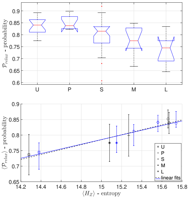
Fig. 7 Top panel: Boxplots of
TABLE 3 Mean (with standard deviation) and median (with the first-25% and third-75% quartiles) values for HZ and
| Assembly level | Mean ± std | Median |
||
|---|---|---|---|---|
| class | HZ |
|
HZ |
|
| U | 15.67 ± 0.53 | 0.839 ± 0.034 |
|
|
| P | 15.66 ± 0.50 | 0.852 ± 0.029 |
|
|
| S | 15.27 ± 0.91 | 0.799 ± 0.067 |
|
|
| M | 15.08 ± 0.65 | 0.775 ± 0.0660 |
|
|
| L | 14.28 ± 0.58 | 0.737 ± 0.0665 |
|
|
Finally, we applied a Kolmogorov-Smirnov (KS-) test to evaluate, with a confidence level set at 90% (or significance level of 0.1), the null hypothesis that the H
Z
or
Table 4: p-values of Kolmogorov-Smirnov test comparing the distributions of H
Z
-entropy (left values) and relaxation probability
| Class | P | S | M | L | ||||
|---|---|---|---|---|---|---|---|---|
| U | 0.958 | 0.500 | 0.417 | 0.024 | 0.065 | 0.024 | 2.003e-04 | 7.725e-04 |
| P | - | - | 0.205 | 0.006 | 0.203 | 0.037 | 7.652e-04 | 9.766e-04 |
| S | - | - | - | - | 0.509 | 0.714 | 7.044e-04 | 0.019 |
| M | - | - | - | - | - | - | 0.148 | 0.243 |
*For galaxy clusters in different classifications. The confidence level for the KS-test was 90%.
6.2 Relation Between H Z and the Cluster Concentration Indices
Apart from the discrete characterization of the assembly state used in the previous sections, one can also probe some continuous parameters, estimated from optical or X-ray data (Carlberg et al. 1996; Girardi & Mezzetti 2001; Zhang et al. 2011; Caretta et al. 2023, and references therein), that are expected to correlate with the evolutionary state of the galaxy system. Here we present, for instance, the concentration indices of a cluster, both from optical galaxy distributions and X-ray from ICM: more relaxed clusters tend to be denser at their centers and have higher values for these indices.
For the optical data, we use the Maximum Likelihood Estimation method (MLE) to determine the optimal concentration indices for the King and NFW radial profiles fitted to the observed projected distributions of galaxies in the clusters of the Top70 sample. The King profile employed for the fitting is the one described by equation (17), while the NFW profile takes the form
where r
s
is the scale radius of the galaxy cluster. The concentration indices of each cluster are related to its respective virial and characteristic radii (r
c
or r
s
obtained by MLE) in the form
Figure 8 shows the relationship between the H Z -entropy and the estimated -cluster- concentration indices for the Top70 sample. The Pearson correlation coefficients between the H Z -entropy values and those corresponding to the indices c K, c NFW and c 500 are 0.448, 0.512, 0.429, respectively. Despite the not strong statistical significance and the remarkable dispersion, an evident growing trend can be seen in the concentration indices with the growth of the H Z -entropy in the systems. This tendency is also subtly manifested in the assemblage classes (represented by the marker symbols in Figure 8): the U and P clusters tend to have higher concentration indices, while the L clusters tend to present lower values of these. S and M clusters appear with a more extended range of concentration indices. It is interesting to note that if we leave only U and P clusters in the above relation, for example for c 500, the correlation increases from 0.429 to 0.603 -these are the typical clusters that appear in studies based on X-rays emission of ICM.
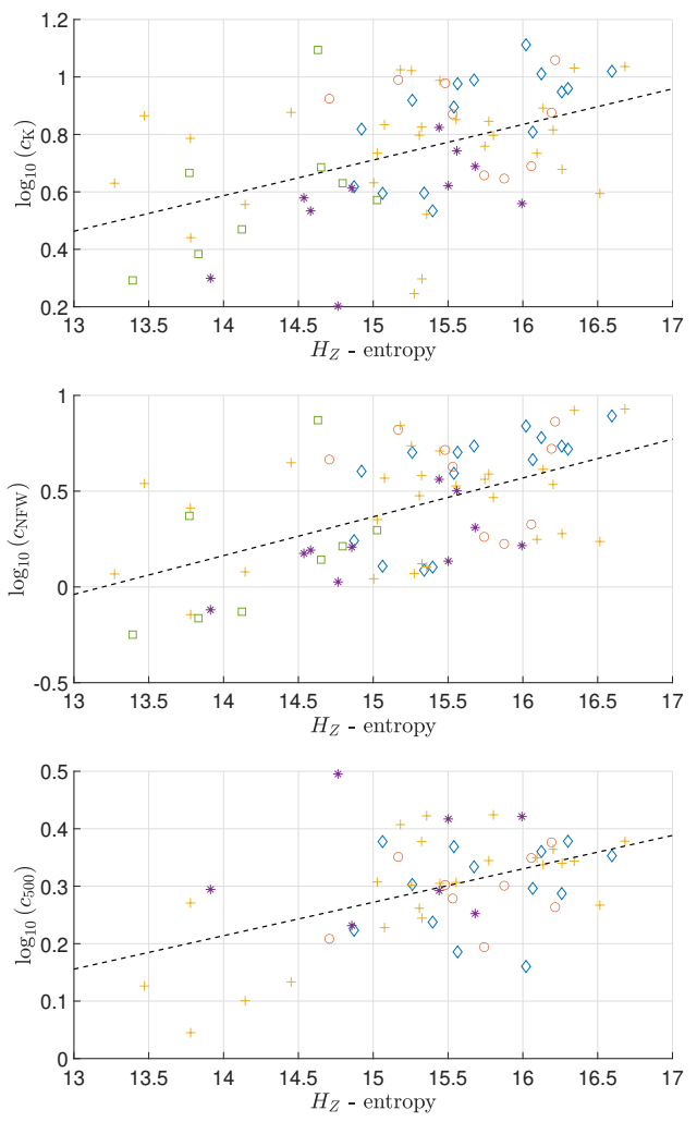
Fig. 8 Scatter plots of H
Z
-entropy vs. concentration indices (c
K, c
NFW, and c
500) for the Top70 cluster sample. The symbols used for the markers have the same meaning as in Figure 5. The dashed line represents the best linear fit to the data, with
We have also probed other continuous dynamical parameters, obtained from X-rays emission of ICM, associated to the evolutionary state of galaxy systems: the concentration c and the luminosity concentration c
L
(resepctively from Parekh et al. 2015; Zhang et al. 2017), the Gini and M
20 morphological coefficients (from Parekh et al. 2015; Lovisari et al. 2017), the substructure level S
C
(from Andrade-Santos et al. 2012), and the C
SB and C
SB4 concentration parameters (from Andrade-Santos et al. 2017). Although the statistics are usually poor, and the aspects captured from X-ray data are not necessarily similar to the ones captured by optical data (which include H
Z
), the results are all similar to the ones showed for
It is remarkable that the only parameter that correlates very well with H Z is r’ c (with a Pearson coefficient of 0.972). The theory states that the natural tendency of a gravitational system towards its evolution is establishing a structure core-halo. This is exactly what the correlation of H Z and r’ c may be suggesting: the core radius grows with the entropy of the cluster.
We consider that H Z is an efficient parameter for estimating the relaxation/dynamical state of galaxy clusters, maybe better than the others we have compared in this incomplete exercise, because it can capture more important aspects of such an evolutionary snapshot. However, it is important to note that no parameter can, alone, account for all the evolutionary aspects, such as interaction with the cosmological environment, collapse and mass growth, galaxy formation, AGN activity, feedback processes, among others, making paramount to consider different observations and analyses for constructing the most complete picture possible.
7 Discussion and Conclusions
In this work we have proposed an entropy estimator, H Z , which can be calculated from global dynamical parameters (virial mass, projected virial radius and velocity dispersion), to characterize the dynamical state of galaxy systems. Initially, a slight modification of the standard T ds Gibbs relation was carried out to include the peculiar behavior of self-gravitating systems and, as a result, an expression was obtained for the entropy component s related only to the galaxy ensemble, which is a function of the internal kinetic energy and the volume of the systems.
The direct association of the H Z -entropy estimator to the dynamical state of the galaxy systems comes from the second law of thermodynamics, according to which entropy increases as the systems advance towards more stable states, reaching a local maximum in virial equilibrium. This does not assert that the galaxy system reaches a stable state of equilibrium, which would be determined by a global maximum of entropy, but rather a state of greater stability than its previous evolutionary configurations, the so-called dynamical relaxation. Thus, although the virial theorem is fulfilled in relaxed states with a local entropy maximum, these are metastable equilibria that can be broken if the galaxy system significantly interacts with its environment, such as through accretions and mergers with other systems. However, if the system is isolated (or its interaction with the environment is negligible), its entropy value remains in the vicinity of the maximum and its behavior in such state will be indistinguishable from dynamical relaxation.
In order to evaluate the power of this entropy to represent the evolutionary state of a galaxy system, we correlated it to four independent estimators: two observational and two statistical. The two observational ones come from analyses of the internal structure of real clusters, particularly the discrete gravitational assembly state (obtained from optical data) and three continuous concentration indices (both from optical and X-ray data), applied to a sample of 70 well spectroscopically-sampled nearby galaxy clusters. The statistical estimators include the Shannon (information) entropy and the relaxation probability, calculated for the same sample of observed clusters and for a sample of 248 halos (simulated clusters) from IllustrisTNG.
The first striking result of our analysis is that the H Z -entropy correlates very well with the gravitational assembly state of the clusters obtained from observational optical data. The H Z -entropy increases with the decrease in the level of substructuring, which is interpreted as the less relaxed a cluster is, the more information is lost when treating it as a virialized system. Specifically, both U and P clusters show the highest entropies, while L present the lowest values for this property. Since P clusters are massive, while possessing only low significance substructures (low mass accretions), they resemble the unimodal U clusters. On their turn, L clusters are, as pointed by Caretta et al. (2023), the ‘less evolved’, in the sense that they are the poorest, less massive and have not suffered significant merging processes yet. S and M clusters present a large range of entropies. This happens because both less or more massive clusters (and both less and more evolved ones) can suffer new mergings or accretion at any time.
The H
Z
-entropy estimator was derived based on specific variables (e.g., per mass unit), which allow comparisons between galaxy systems of different masses (
A possible evolutionary line between systems at different assembly levels has been schematized in Figure 9. Multimodal (M) systems could be formed by the merger of two or more low-mass unimodal (L) systems. These mergers increase the entropy level of the systems due to the increase in mass and number of particles (i.e., galaxies). As gravity further assembles the fused parts, a main structure is formed in the clusters, and, when still dynamically significant substructures remain, we have substructured systems (S). In this process, the entropy increases because the main structure, which is larger than the rest of the substructures, begins a virialization process and dominates the dynamics of the cluster. The substructures are special configurations in the distribution of galaxies, macroscopic movements that can slightly affect the dynamics of the system. However, these are little by little accreted and dissolved by the main structure, until they become less significant and the clusters evolve marginally towards the more assembled states primaries (P) and unimodals (U), where the entropy is greater given the large homogeneity of the distribution of galaxies, large velocity dispersion and the proximity to virialization.
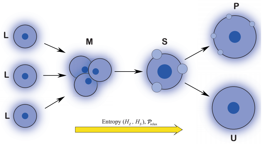
Fig. 9 Diagram of a possible evolutionary line between systems in the different assembly levels (U-P-S-M-L). The entropy levels of the galaxy systems, obtained using the H
Z
and H
S
estimators, increase as they progress towards more dynamically relaxed states (with a higher probability of relaxation,
It is important to highlight that, despite the notable tendency of H
Z
-entropy to increase with the L
Resuming the question about unimodal clusters, we have also verified that L clusters lack the core-halo spatial configuration, unlike U clusters that exhibit a clear central concentration of galaxies. In fact, as can be seen from the galaxy concentration indices, U clusters generally achieve the highest concentration indices while L clusters have the lowest. Thus, the Hellinger distance between the respective observed and relaxed PDFs of a cluster becomes larger when the latter lack a central concentration.
Concerning the statistical estimators we used to test H Z -entropy, we found that the Shannon -or information- entropy H Z presents a remarkable (almost linear) correlation with it.
Information entropy does not necessarily have a simple correspondence with physical entropy, but we can provide a possible explanation for the correlation between the H
Z
and H
Z
entropies as follows. Given that the cylinder of x-points of observational data constitutes a projected phase-space (e.g., it contains 2D-position and 1D-velocity coordinates of particles in a system that evolves with time) for each cluster,
On the other hand, the argument
This interpretation is reinforced by the relaxation probability
The entropy estimations presented here are very promising because, once one has a representative sample of galaxy members for the cluster, the calculation of the input parameters is straight forward. This low-cost analysis is much easier than the broader one presented in Caretta et al. (2023), and can also be used as a complementary analysis in the study of the assembly state of the galaxy systems. It is still lacking a deeper analysis of the implications of the results presented here, which we plan to do in a future work. We also intend to extend this analysis to other scales of galaxy clustering, especially in the direction of the evolution of the large scale structures like the superclusters of galaxies.
Our main conclusions are the following:
• The H Z -entropy estimator, which depends solely on observational (optical) parameters, adequately captures the entropy of clusters manifested in the (spatial and velocity) distribution of their member galaxies.
• The H Z -entropy is related, through the second law of thermodynamics, to the evolutionary state of galaxy systems. Entropy increases as systems evolve towards more stable states, reaching a local (non-unique) maximum at virial equilibrium.
• There is a significant correlation between the H Z -entropy of galaxy systems and their gravitational assembly states (A, Caretta et
al. 2023), presenting an entropy growth in the L
• There is a remarkable (almost linear) correlation between H Z -entropy and the Shannon (information) entropy, H S , reinforcing that the dynamical entropy we propose can capture the increase in disorder and loss of information in the process of virialization.
• Clusters with higher velocity dispersions of member galaxies tend to have higher H Z and H S entropy values, indicating more random galaxy distributions.
• The H Z -entropy estimator shows a great capacity to capture the state of relaxation and evolution of the galaxy systems, maybe better than the one presented by other conventional continuous parameters used for this purpose.
• The H Z -entropy estimator provides valuable information on the dynamical state and assembly levels of galaxy clusters, which may have significant applications in studying the evolution of galaxy systems and understanding their dynamics.

