


 nueva página del texto (beta)
 Inglés (pdf)
 Artículo en XML
 Referencias del artículo
 Enviar artículo por email
 Citado por SciELO
  Similares en
SciELO
Similares en
SciELO 
 Permalink
1 Introduction
Transient events are phenomena with a short lifespan when compared with everything else in the universe. However, since their behavior and duration can vary from one object to another, they present a great diversity, even within same class of events. Gamma ray bursts can last less than a second while microlensing or supernovae events remain visible from a few days to several weeks.
Type Ia supernovae (SNIa) are among the most important types of transients for cosmological analysis. This particular type of transient has been key for the determination of the expansion history of the universe by comparing the observed flux of these objects with their redshifts. Thanks to SNIa, the recent acceleration of the universe expansion has been derived and measured [Riess et al.(1998), Perlmutter et al.(1999), Betoule et al.(2014)].
With the advent of more powerful and complete all-sky photometric surveys, either from ground telescopes or satellites, an increasing amount of data will be delivered to the scientific community. This enormous volume of data requires more sophisticated and efficient methods to analyze them and report important findings, such as SNIa. The more data modern telescopes are capable of gathering, the more latent is the necessity of algorithms, big data techniques and automation strategies to fully study and leverage such amount of information.
Dedicated rolling search has been employed in several surveys to search for transients in specific regions of the sky and to perform photometric follow-up of these events. Some of these surveys are the Supernova Legacy Survey (SNLS) [Guy et al.(2010)], the Panoramic Survey Telescope and Rapid Response System (Pan-STARRS) [Scolnic et al.(2018)], the Sloan Digital Sky Survey (SDSS) [Sako et al.(2018)], the Hyper Suprime-Cam Subaru Strategic Program (HSC SSP) [Aihara et al.(2018)] the Dark Energy Survey (DES). Smith et al. (2020) have developed programs in search of SNIa.
The Vera C. Rubin Observatory Legacy Survey for Space and Time (LSST) is one of these surveys whose objective is to provide an unprecedented volume of images and information, using the largest digital camera ever constructed [IveziÀet al.(2019)]. Along with the LSST, there is an important effort to provide a software backbone for the processing and generation of LSST data in the form of the LSST Science Pipelines, the LSSTsp, for short [Jurić et al.(2017), Bosch et al.(2018)]. The LSSTsp is a suite of software packages capable of enabling the creation of dedicated data products with high quality and great performance [Axelrod et al.(2010)]. This is the base tool the LSST survey will use to accomplish its science goals and that this work employs to analyze and study SNIa in real and simulated images.
Other surveys have developed tool sets to analyze transients. For instance, [Perrett et al.(2010)] developed a pipeline for SNLS that involved calibrating, warping and subtracting the images; then using photometry fittings; and finally, generating triplets of transient candidates that were visually confirmed by experts, relying on manual classification.
Another example is [Kessler et al.(2015)], which described the DES-SN difference imaging pipeline used to detect transients for DES . This pipeline is based on selecting objects, mixing thresholding images and matching catalogs. They use Hotpants [Becker(2015)], an implementation of the Optimal Image Subtraction (OIS) [Alard Lupton(1998)], and Autoscan, a machine learning code to replace human intervention when identifying transient objects [Goldstein et al.(2015)].
Recently, [Sánchez et al.(2022)] worked using a difference image pipeline built on the LSSTsp to analyze simulated images that included SN Ia light curves. It also measured cosmic distances and cosmological parameters from the SNIa to monitor the detection efficiency of the LSSTsp. [Sánchez et al.(2022)] employed the LSSTsp systems as a tool to study images from different characteristics for the needs of current and future surveys.
As powerful as difference imaging is, recent works have also leveraged machine learning to further refine the detection transients. For instance, [Goldstein et al.(2015)] proposed a random forest approach to identify artifacts among the objects extracted from difference images in the DES-SN transient detection pipeline [Kessler et al.(2015)]. Their method presented a missed detection rate of 5% and a false positive rate of 2.5%.
An example of classification of detected transients within the LSST comes from [Pasquet et al.(2019)], which proposes a complex deep learning architecture to characterize and classify supernovae of different types, based on previous applications of the same strategy to other similar problems in astronomy. They tested it with simulated data from the Supernova Photometric Classification Challenge SNPhotCC, which is a set of simulated supernovae on DES images [Kessler et al.(2010)]. This algorithm presents an accuracy of over 86% for SNPhotCC with an AUC of0.937, and despite some uncertainties, it obtained an accuracy of between 90% and 97% with an AUC of between 0.990 and 0.997 for simulated SNIa in the LSST Deep Fields.
Another example comes from [Boone(2019)] which proposed Avocado: a Gaussian process augmentation applied over light curves in all bands, used to train a decision tree to classify different types of transients for the Photometric LSST Astronomical Time-Series Classification Challenge or PLAsTiCC [The PLAsTiCC team et al.(2018)]. PLAsTiCC is a community-wide challenge to foster the development of machine learning classification algorithms on a set of realistic LSST simulations of transient events. Avocado was the winner of this challenge, achieving an AUC of 0.957 for the classification of SNIa.
Lastly, [Neira (2020)] used a Random Forest based classification for binary classification (transient/non-transient) and eight-class classification. We use their approach with their base features as well as some modifications to understand the relevance of the studied additions.
In this paper we present a study of detection techniques to select SNIa on images from big telescopes. To obtain and analyze our results we use the LSSTsp. Our main objective is to show how it is possible to explore and design procedures that contribute to the exploration and analysis of data for the astrophysics field through the use of powerful computational tools.
2 Materials
This section presents the characteristics of the images used to test the proposed pipeline. We employ real data and try to find genuine supernovae present in the images. We also work with simulated data, creating and injecting supernovae in the input images, to help us understand the behavior of the different tasks with varying inputs. As these new images are virtually equivalent to normal acquisitions, we can use them as inputs to determine the sensitivity of our processing by counting the SNIa detected after simulations, as if these were real phenomena.
2.1 Real Data
We employ two types of real data: images obtained from the Canada France Hawaii Telescope (CFHT) and light curves from SNIa found in these images by the Supernovae Legacy Survey (SNLS). The SNLS has developed a major program on supernova detection that includes an image processing pipeline. It has detected more than 300 SNIa in its first five years of observation [Guy et al.(2010)].
2.1.1 Images
Images from CFHT datasets belong to one of the four deep fields (noted D1, D2, D3 and D4) during the first three years of the survey: the D3 field. We use this field as a limited sample that allows us to test our contributions within the limits of our technical resources. These first three years, from 2004 to 2006, have available valuable results regarding the detection of SNIa among the images [Guy et al.(2010)]. These images are obtained using the Megacam camera. The Megacam has 36 charge-coupled devices (CCD) capable of providing an image. The number of images per filter varies as shown in Table 1; the total number of images in the used field is 54614. It is noticeable that most images use filters r and i, which justifies why we focus some of our results on the former.
Table 1: Total of original CCDs images per filter for the first three years of CFHT observation in field D3
| Filter | Number of images |
|---|---|
| r | 13242 |
| i | 18033 |
| g | 10828 |
| z | 12511 |
These deep fields have the following characteristics:
• An observation set every 5 nights on average.
• When a night is observed, 5 observations are gathered on average.
• 1 deg2 of sky observed during almost 6 consecutive months every year.
• A full focal plane composed of 36 CCDs.
• Each CCD is
• Each pixel is 0.186 arcsec.
• The limit magnitude of four fields are u = 27.5, g = 27.7, r = 27.4, i = 27.4 and z = 26.2.
• Depth per night is about magnitude 3.
• Seeing range between og approximately 0.6 and 1.1 with an average of 0.8
2.1.2 Light Curves
To validate our results, we use the SNIa reported by the SNLS and identified using spectroscopy. This survey has identified and measured the photometric properties of 252 SNIa with a redshift range of between 0.15 and 1.1 [Guy et al.(2010)] and reported at least 485 SNIa candidates [Bazin et al.(2011)]. The first SNLS sample provides one of the most uniform sets of SNIa available, but the actual number of objects per deep field is low, providing only 75 SNIa for the D3 field in the three years of observation. Nevertheless, these supernovae serve as the ground truth for the detection.
2.2 Simulated Data
We present here the simulation of SNIa injected on real images. We simulate type SNIa through the Supernova Analysis Software or SNANA [Kessler et al.(2009)] using the Spectral Adaptive Lightcurve Template 2 model, also known as SALT2 [Guy et al.(2007)], and then inject them into the CFHT images, to create an effective sample of time series for testing our analysis using machine learning algorithms along with Poisson noise from the source. We generate 5000 SNIa for the CFHT deep field D3, and we inject each one on the successive visits during the season and the field. Each injection is individually given a coordinate in the images and then added to it.
We inject simulated point sources on real CFHT images. We choose a random date and a random location from the CFHT image set to inject the simulated supernovae. The selection of the random location is achieved by employing an external catalog to select any galaxy in the field as a host. This external source catalog provides the location of galaxies within a sequence of images. At this point, all injections are then handled as single image simulations: we locate the coordinates of such galaxy in the map of the sky so we know which images we need to retrieve. Subsequently, we get the respective image in the located coordinates for every observation in the simulated curve. After that, we calculate the local PSF values using principal component analysis to give shape to the supernovae; then we inject the simulated supernovae with an intensity added to that of the host galaxy, with a random off-set to the location within the confines of the host galaxy.
3 Methods
We use the LSSTsp as the base tool to detect the SNIa. We present in this section the main tasks used and some custom tasks we developed for our specific needs.
3.1 The LSST Science Pipelines
The LSST Science Pipelines (LSSTsp) was developed for the purpose of processing data for the Vera C. Rubin Observatory Legacy Survey for Space and Time. It is developed in Python and C++ [Kantor et al.(2007), Bosch et al.(2018)] and it has being tested through data challenges with different levels of complexity and being constantly prototyped. Currently, it has more than 40 packages that perform a large variety of image and data processing operations; it includes efficiently designed C++ algorithms wrapped in SWIG. It provides architectures to process inputs and to generate the required results [Ivezić et al.(2019)].
The LSSTsp has several different tasks for image processing. Each task has its own independent responsibilities, but when put together, it is possible to employ the intermediate products to detect transients by means of a pipeline. Our work relies on the LSSTsp v14 for assembling a processing pipeline for SNIa detection, through the use of some Difference Image Analysis (DIA) tasks and routines. We acknowledge that more recent versions of the LSSTsp have included new features related to the analysis presented in this paper, but we still use this version to ensure compatibility with our previous work and this does not change the relevance of our results.
As there is not an official transient detection pipeline for CFHT images within the LSSTsp, we assemble one as a starting point. This pipeline is shown in Figure 1. It has three main stages: First, the Generation of Difference Images, which encompasses the pre-processing, coaddition, and subtraction of images using the OIS. The second stage is the Candidate Selection, which comprises the optimization of the detection of sources in the difference images, the association of sources to produce multi-channel source associations (up to 5 pixels) to produce light curves, and the selection of transient candidates based on their light curves. In this stage, all operations that use the difference image are noted with the prefix DIA (Difference Image Analysis). The third and last stage is the Type Ia Supernova Identification, which applies a machine learning algorithm to the candidates to recognize the SNIa.
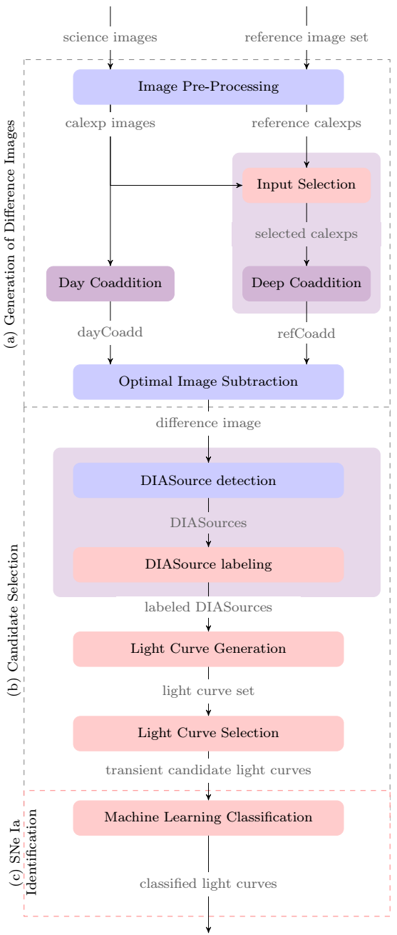
Fig. 1 The Supernova Detection Pipeline divided in three stages: (a) Generation of Difference Images; (b) Candidate Selection; and (c) SNe Ia Identification. Blue tasks are left untouched, purple tasks have been modified and red ones are tasks we created for the LSSTsp. The color figure can be viewed online.
Figure 1 highlights elements that we use, adapted and created for the pipeline. Tasks in blue are used without any modification, tasks in purple have been extended to help them fit better into the new pipeline. Tasks in red are new and they are programmed using the task architecture of the LSSTsp and developed completely to answer the need of processing for particular points of the pipeline.
3.2 Generation of Difference Images
The purpose of this stage is to generate the difference images for each reference and science image input. As shown in Figure 1a, the tasks involved in this stage are the Image Pre-processing; the Image Coaddition tasks (Day Coaddition and Deep Coaddition tasks) to generate the respective input images for the image subtraction; and the Optimal Image Subtraction itself. Here we study the impact on the existing software of implementing a task to select better reference images (calexps) for the Deep Coaddition.
3.2.1 Image Pre-Processing Task
Firstly, the Image Pre-Processing task encompasses the calibration of the initial exposures, the artifact correction, the detection of visible sources, and the masking of saturated and edge pixels. This processing provides a relatively clean set of images with noise corrections, masked saturated pixels and cosmic rays. These images are used as inputs for the Image Coaddition tasks. The result of this first task is a set of calibrated exposures or calexps.
3.2.2 Image Coaddition and Input Selection
Typically, when using coadditions in LSSTsp, the final user is in charge of selecting calibrated exposure inputs and there are no enforced rules within the code to differentiate between a coaddition for a reference image and one for a science image. This process is reached through the use of two tasks and it is indifferent to the purpose of the output. In the pipeline, we opt to fuse both generation and assembly tasks together and then specialize each one to generate the coaddition for science and reference calexps. We call these the Day Coaddition and the Deep Coaddition tasks. This allows us more control over each process independently, without affecting the other. From a technical perspective, this also mitigates the impact of bottlenecks for global field processing and allows the new tasks to be more time efficient when generating the deep coadditions.
Selecting high quality inputs is vital to ensure a good coaddition and subsequently good difference images. Using low quality inputs without any sort of quality metric has the potential of propagating noticeable errors and aberrations from the coaddition, all the way to the detection of transient candidates. Errors on the images come from the sky background and increase as the square root of the signal, bad atmospheric conditions or deficient seeing. As the image subtraction operation alters the inherent noise of the inputs through convolution, they become problematic and the artifacts become more visible most of the time. We choose to address this issue for deep coadditions.
Day Coaddition Task
The objective of this task is to generate a high quality science coaddition image, as mentioned before. Day coadditions, or dayCoadds, are built by using the different exposures acquired on a given night. As there is a limited number of acquisitions per night (between 4 and 10 in most cases), we use all available exposures to ensure the best possible quality without performing a selection of high quality inputs. This way of generating day coadditions means that very short-lived objects (less than one night) are not registered in the detections or might appear as single point detections.
As with science images, we expect the transient and variable objects to be present here; thus, when performing the OIS, we match their PSF to that of the astrometrically corresponding deep coaddition to detect them after subtracting both.
Deep Coaddition Task
Deep coadditions created from a reference image set are referred to as refCoadds. These coadded exposures, which come from a wider time frame belonging to an outside acquisition year, help to detect all changes in science images during the subtraction. As explained before, the convolution Kernel that calculates the OIS when matching with the day coaddition modifies these images. High quality images provide better and less complex PSFs to be parametrized by the sum of Gaussians via the OIS, reducing the overall artifacts later when a subtraction is performed.
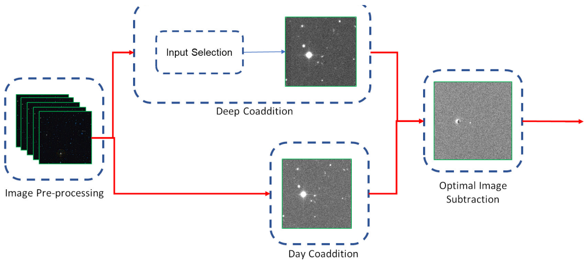
Fig. 2 First part of the pipeline: the generation of difference images. The tasks here are responsible for generating the reference and science image coadditions, and then performing the subtraction using the OIS algorithm. The Deep Coaddition task generates the reference image, whereas the Day Coaddition task creates the science image. The Image Subtraction task generates the difference image as final result.
Ensuring the quality of the inputs is especially important when constructing the deep coaddition, because input datasets for these can span up to hundreds of different images acquired during several months of operation. Therefore, we construct these references guaranteeing high signal-to-noise on the result and thus obtaining high quality difference images. To achieve this, we perform an selection using the noise variance levels on the input images after warping and adjusting them to their respective patch in the skymap, but before assembling the final coaddition. As noise levels change locally within the image and can present variation between the original calexps and the smaller patches used for the coaddition, it follows that the optimal approach is to use the values in the patches as criteria for the selection. We call this process the Input Selection.
3.2.3 Optimal Image Subtraction
As already mentioned, we use the OIS [Alard & Lupton(1998), Alard(2000)] LSSTsp task with the new dayCoadds and refCoadds as inputs. We use the default parameters of 3 Gaussians with degrees 4, 2 and 2. As expected, the OIS generates a difference image that is the output of the current stage and will be the input of the next one
3.3 Candidate Selection
The main objective of this stage is to produce a set of plausible candidates, from the detections in the difference images, to be transient objects. The tasks involved in this stage are the DIASource Selection, the Light Curve Generation and the Light Curve Selection. These tasks are shown in Figure 1b. We perform a quality analysis for the sources detected in the difference images through the use of footprint analysis.
3.3.1 DIASource Selection
This first task of this stage is divided in two phases: The DIASource detection and the DIASource labeling.
DIASource Detection
The detection of sources in difference images is performed using the default single frame measurement algorithm of the LSSTsp that searches positive and negative local peaks, and using a detection threshold of
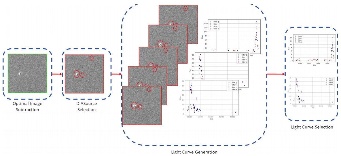
Fig. 3 Second part of the pipeline: Light curve detection and selection. The tasks here include the detection of DIASources; and the detection and selection of light curves.
Previous analysis using the LSSTsp suggest that an underestimation of noise in the CFHT images ends up generating a high number of detections during this step [Slater(2016)]. To mitigate this, we re-estimate the value of background noise on the images using the algorithm in the LSSTsp and then recalculate the threshold value defined for the image in the given band. This process, even if time-consuming, ensures that there are less bogus detections in the images, and guarantees that the noise is not inflated.
When a DIASource is detected, one or two footprints are calculated on a
where R’ is the result of a region growth over an initial group of pixels R + or R - such as:
Here,
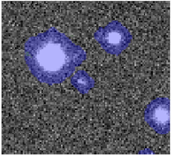
Fig. 4 Example of sources with footprints overlaid as semi-transparent blue groups of pixels. The color figure can be viewed online.
R + and R - are initial groups of at least 5 pixels for which:
Here th is the threshold value, and x and y represent the pixel coordinates.
Notice that, as the region growing algorithm determined by equation 3 does not take into account pixel values, footprints F + and F - can have intersections.
DIASource Labeling
Once the footprints of a DIASource are calculated, the number of pixels and their flux are measured. These values are used to label the corresponding DIASource. The analysis of DIASources is a custom task independent from similar ones currently present in more recent versions of the LSSTsp such as DipoleAnalysis. The possible labels that we assign are:
• Positive: DIASources that only have F +. Their presence is the result of a transient object in the science image.
• Negative: DIASources that only have F -. These are rare residuals and they sometimes indicate transients present in the reference images.
• Dipole: DIASources with F + and F - with balanced flux and size with low geometric overlapping.
• Fringe: DIASources with F + and F - with balanced flux and size with high geometric overlapping.
• Artifact: DIASources that do not fit in any of the previous categories.
Let us define:
To determine whether a DIASource is a Dipole or a Fringe, we define two properties: Geometric Dipoles
A Geometric Dipole
A Photometric Dipole
Therefore, using the properties defined in equations 7 and 8, we define a Dipole
And a Fringe
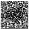
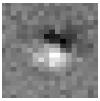
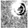
To summarize, we evaluate the amount of overlapping in terms of pixels and calculated flux to determine the label for a given footprint. The proportions are empirically determined, leaving the possibility of a more in-depth study and refinement of these categories. Visual examples of their aspect are presented in Table 2.
TABLE 2 Footprint labels defined for every source detection based on their footprints*
| Label | Visual Aspect | Description |
|---|---|---|
| Positive |
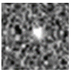
|
Sources that only have positive footprints. Their presence usually is the result of a transient object in the science image. |
| Negative |
|
Sources that only have negative footprints. These are rare residuals and they sometimes indicate transients present in the reference images. |
| Dipole |
|
Sources with positive and negative footprints. These artifacts occur when there are alignment problems between the images. |
| Fringe |
|
Sources with positive and negative footprints. These artifacts occur when there are inaccuracies in the PSF matching algorithm. |
| Artifact |
|
Sources with both positive and negative footprints, but that do not fall in the Dipoles or Fringes categories. |
*The Visual Aspect column shows a general idea of the type of objects labeled as such.
3.3.2 Light Curve Generation
From the detected and labeled DIASources obtained from the previous step, we match all DIASources that are located at the same coordinates within a 1 arcsec of radius in all the different images along all the seasons, under the assumption that all these detections belong to the same object. For each set of matched DIASources, we build a light curve and assign an object ID to it. Consequently, each light curve may be composed of several DIASources and always has at least one.
The output of this task is a catalog of the light curves for every filter. Each light curve is stored as set of DIASources with all the relevant information such as the coordinates, flux, error, magnitude, filter, and date (MJD format). The study of the DIASources and its classification is helpful to identify which type of object is being described by the light curve.
3.3.3 Light Curve Selection
A consequence of the previous task is that a detected light curve can technically contain, in the worst case, a single point. Isolated detections of an object do not strongly indicate the presence of supernova-like transients; in fact, they can be indicative of anomalous subtractions, short-lived events, or transients who vary in intensity and position at the same time. The Light Curve Selection task is implemented so that it chooses only curves that satisfy two criteria: at least five total detections and data present in at least two different bands. This ensures that the object has a certain continuity between observations and that its residual light intensity can be picked in different bands.
Although these criteria might appear to be simplistic, they perform a considerable reduction of the candidate set, while also being conservative enough not to reject true transients.
3.4 Type Ia Supernovae Identification
The final stage of the pipeline classifies the transient candidate light curves to identify real SNIa, using the machine learning classification method proposed by [Neira (2020)]. Figure 1c depicts this task in the pipeline. We use the identification part of the pipeline to validate the impact of our studies and characterization, specially when introducing new variables calculated after obtaining better quality light curves.
Regarding the identification, we worked on four fronts: First, the adaption of the method to binary classification (SNIa and non-SNIa). Secondly, the selection of relevant data features and the introduction of three new ones in the form of the
Before classifying, the method uses dimension reduction via feature extraction. Light curve observations are not sampled at regular intervals and all of them do not have the same number of observations. This makes it very challenging to use the time-series data directly for classification using traditional methods. To solve this difficulty, a set of characteristic features is extracted from each light curve instead, using statistical and model-specific fitting techniques. From the original implementation, we only use 23 features that are strictly geometrical and statistical (Table 3). These features are categorized in the following four groups: moment-based, magnitude-based, percentile-based and fitting-based.
TABLE 3 Features calculated for machine learning training of light curves
| Feature | Category | Description |
|---|---|---|
| skew | moment-based | Asymmetry of the curve |
| kurtosis | moment-based | Measure of extreme values in either tail of the curve |
| small kurtosis | moment-based | Small sample kurtosis |
| std | moment-based | Standard deviation |
| *beyond1std | 2*moment-based | Percentage of magnitudes beyond one standard deviation from the weighted mean. |
| Each weight is calculated as the inverse of the photometric error | ||
| stetson j | moment-based | The Welch-Stetson J variability. A robust standard deviation |
| stetson k | moment-based | The Welch-Stetson K variability. A robust kurtosis |
| max slope | flux-based | Maximum absolute slope between two consecutive observations |
| amplitude | flux-based | Difference between maximum and minimum intensity |
| median absolute deviation | flux-based | Median discrepancy of fluxes from the median magnitude |
| median buffer range percentage | flux-based | Percentage of points within 10% of the median flux. |
| pair slope trend | flux-based | Percentage of all pairs of consecutive positive slope measurements |
| *pair slope trend last 30 | 2*flux-based | Percentage of the last 30 pairs of consecutive positive slope measurements |
| minus percentage of last 30 pairs of consecutive negative slope measurements. | ||
| resPos | flux-based | Percentage of footprints labeled as positive in light curve |
| percent amplitude | percentile-based | Largest percentage difference between absolute max. magnitude and the median. |
| percent difference flux percentile | percentile-based | Ratio of F5,95 and the median flux. |
| flux percentile ratio mid20,35,50,65,80 | percentile-based | Ratio of percentile and F5,95 |
| poly1_a | fitting-based | Coefficient of the monomial curve fitting |
| poly2_a,b | fitting-based | Coefficients of the quadratic curve fitting |
| chi2SALT2 | fitting-based |
|
| chi2sGauss | fitting-based |
|
The three new features we introduce are:
• The
• The
• The percentage of DIASources labeled as positive present in the light curve of a given object, denoted as resPos. This feature is obtained by calculating the number of footprints labeled as positive as a percentage of the total number of sources present in the light curve.
4 Results
We present here the results of our analyses in each stage using our pipeline: Generation of Difference Images, Candidate Selection, and Type Ia Supernova Identification. We show the results when applying the different options offered by the pipeline.
4.1 Tuning the OIS
We tested the effect of modifying the OIS parameters to better adapt it to our input images using the simulated inputs with various fluxes. Among the many parameters that can be tuned to optimize the OIS, we varied the cell size, the Spatial Kernel Order and the number of Gaussians used to model the PSF for different patches in the images and then we applied a grid search test to find the better parameter combinations. For the cell size, we tested values between 50 and 500 pixels, we varied the number of Gaussians between 3 and 8 and for the Spatial Kernel Order we used several combinations of degrees between 1 and 9. There were no improvements of more than 1.2% in the number of detections. For all the studied parameters, we concluded that the default values fixed by the Rubin Observatory Data Management team are the optimal ones for our data as well (real CFHT data with simulated supernovae).
4.2 Generation of Difference Images
To measure the impact of the pipeline different options on the Deep Coaddition task, we compared the number of DIASources detected on the CFHT image dataset with and without input analysis and then we analyzed the quality of such sources using the footprint labeling. Figure 6 presents the number of detections as a function of the number of input coadded images in three situations: (a) when using Input Selection to select low variance images, (b) when selecting random input images, and (c) when averaging the results for several images while using low variance, high variance, and without Input Selection (noted as random). Figure 7 shows the same results, but instead of variance, it depicts Input Selection based on PSF radius size. From these results, we infer that the number of detections in coadditions is reduced when selecting input images with low variance and low PSF radius size.
Fig. 5 Comparative percentage of labeled DiaSources. Not only does the original pipeline have more detections, but the proportion of spurious detections (non-positive) is consistently higher that when using Input Selection. The color figure can be viewed online.
Fig. 6 Analysis of the number of detections with different amounts of coadded images using Input Selection to coadd images with: (a) low variance inputs and (b) random variance inputs. (c) Analysis of the number of average detections for low, high and random variance input coadded images. Image ID indicates the location of the image in the skymap. The color figure can be viewed online.
Fig. 7 Analysis of the number of detections with different amounts of coadded images using Input Selection to coadd images with: (a) low PSF Radius inputs and (b) random PSF Radius inputs. (c) Analysis of the number of average detections for low, high and random PSF Radius input coadded images. Image ID indicates the location of the image in the skymap. The color figure can be viewed online.
We can consider that the higher the number of DIASources detected, the more spurious detections are present among them. As such, a precise pipeline should strive to reduce the overall number of detections while preserving real transients. Consequently, better coadditions should have fewer detections with unchanged efficiency of detecting transients. The efficiency of detecting transient is evaluated with the simulated data and does not vary significantly with the coaddition. Our results show that increasing the number of input images for the coaddition reduces the number of detections as well.
By Input Selection and DIASource analysis, we were able to reduce the overall source detection density for one filter as shown in Table 4. This represents a reduction of 80% of detections, a percentage that is greater if other filters are taken into consideration. This result is comparable with the artifact density found by [Sánchez et al.(2022)], which also uses a strategy to ensure high quality template images, with the difference that we use straightforward modifications with real data.
Table 4: Number and density of source detections before and after input selection on filter r
| Number of Sources | Sources per square degree | |
|---|---|---|
| Before input selection | 4215406 | 48452.9 |
| After input selection | 87042 | 1000.5 |
Another measure of the impact of our contributions is the proportion of positive and dipole labeled DIASources. Firstly, we obtained around 85% of positive labeled DIASources, against only 24% before our additions. We were also able to reduce the number of dipoles from 40% to 9%. Similar reductions in artifacts and fringes are measured, as illustrated by Figure 5.
By enhancing the quality of the inputs we reduce the total number of detections while yielding higher quality transient-like candidates.
4.3 Candidate Selection
We present the results of selecting SNIa candidates in the pipeline with the different options presented with simulated and real data.
Real data
When we tested our pipeline with real data (CFHT images), it preserved among the candidates 85% of the supernovae reported by SNLS (64 out of 75).
We also determined the quality of the supernova-like candidates by measuring the proportions of DIASource labels per object. Results on the CFHT images show that, before Input Selection, at least 33% of the objects presented light curves with 70% or more detections labeled as artifacts, whereas after the Input Selection only around 6% presented this property. For the dipoles, the difference was less stringent, as some of the built light curves still had a mixture of dipole and positive detections, that can be probably attributed to subtraction problems and other imaging issues.
Before Input Selection, the distribution of positives per light curve was so low that there were no strong candidates with this quality. Our results show that 72% of the light curves have 80% of DIASources labeled as positive. The reduction of the number of artifacts with the extra options of the pipeline is notable: originally, at least 33% of objects we obtained have light curves with 70% or more detections that were labeled as artifacts, whereas for our pipeline only less than 1% presented this quality.
Simulated Data
In the case of simulations, we tested the Candidate Selection by injecting 5000 artificial supernovae. While obtaining 80% less total detections, we were able to find 75% of the injected supernovae. By creating simulations that avoided injecting SNIa too near the edges of patches we were able to increase the number of found SNIa to between 75% and 78%. The detection efficiency drops at a redshift of about 0.8.
Figure 8 illustrates that most of the light curves that were not found by the algorithm have a low number of individual points and a considerable number of high magnitude points. These qualities make these curves more susceptible to be missed, thus reducing the overall efficiency. By using curves with points with a lower magnitude, and a slightly higher number of points, we improved the pipeline’s response to the simulated events.
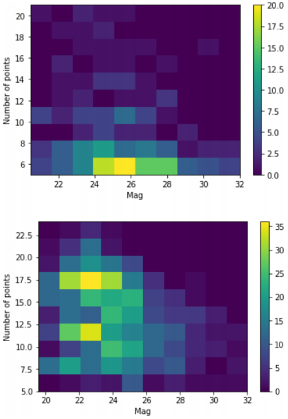
Fig. 8 Heatmap of light curves per configuration of maximum magnitude values vs number of points for the simulated curves that were not found (Top) and the simulated curves that were successfully found by the algorithm (Bottom). The color figure can be viewed online.
The results in this case are highly dependant on the simulated curves and the magnitude used. It is possible to vary the threshold to allow more candidates, at the cost of more spurious candidates.
The distribution of positive residuals among the simulated type Ia supernova light curves showed that 95% of these detected supernovae had at least 90% or more of their individual detections labeled as positive residuals. Thus, they have an overall higher quality and demonstrate that we are able to obtain a cleaner candidate set.
It is important to notice that, even if we are able to greatly reduce the load by sacrificing some accuracy, other works provide better insights on how to improve these results. For instance, [Goldstein et al.(2015)] use machine learning methods to reduce by 11% the load of candidates to evaluate with a loss of only 1%. We also believe that an adapted threshold for detection might mitigate this loss, at the cost of augmenting again the number of candidates.
Given the fact that the proportion of positive labels among all objects rose in the light curves we obtained, we assert that our enhancements go in the right direction. Reducing the number of DIASouces and increasing their quality provides a more accurate detection of transients. This accuracy is not only susceptible to increase by applying methods to automatically classify SNIa, but also when using high quality datasets with strategies such as Input Selection.
4.4 Type Ia Supernova Identification
In order to assess the efficiency of the algorithm to classify candidate light curves in two classes, SNIa or non-supernova objects, we used:
• A balanced training set composed of 1333 simulated light curves of each class (simulated SNIa and real non-SNIa light curves).
• An unbalanced validation set that contains 1404 simulated supernovae and 444 real non-supernova light curves randomly selected from photometric classification from previous analyses. Table 5 shows the classification results for this set.
• A second validation set consisting of 130 real SNIa light curves and 444 real non-supernovae light curves. To supply the real SNIa light curves we use the 75 real SNIa instances detected by SNLS and then we oversampled to generate the remaining ones using the technique described by [Neira (2020)]. Table 6 depicts the results for this set.
TABLE 5 Results of the machine learning binary classification of supernovae and non-supernovae objects*
| Test | F1-score | Precision | Recall | AUC |
|---|---|---|---|---|
| Base features in filter r | 0.899 | 0.853 | 0.950 | 0.983 |
| All features in filter r | 0.911 | 0.883 | 0.941 | 0.984 |
| Base features in all filters | 0.951 | 0.958 | 0.943 | 0.995 |
| All features in all filters | 0.960 | 0.970 | 0.949 | 0.996 |
*Using simulated data: 1404 simulated supernovae and 444 real non-supernova light curves.
Table 6: Results of the machine learning binary classification of supernovae and non-supernovae objects*
| Test | F1-score | Precision | Recall | AUC |
|---|---|---|---|---|
| Base features in filter r | 0.744 | 0.690 | 0.807 | 0.968 |
| All features in filter r | 0.754 | 0.650 | 0.900 | 0.971 |
| Base features in all filters | 0.901 | 0.926 | 0.876 | 0.996 |
| All features in all filters | 0.918 | 0.891 | 0.946 | 0.997 |
*Using real data: 130 oversampled instances of 75 real supernovae and 444 real non-supernova light curves.
The classification algorithm had an f-score of 0.899 and 0.744 on simulated and real data respectively, using only the original base features proposed by [Neira (2020)]. When using the base features, the features we added and light curves with detection on several filters, we went from an f-score of 0.911 and 0.901 up to 0.960 and 09.18 for simulated and real data respectively. In both cases there was a slight improvement in the classification performance.
We also calculated the comparative ROC curves for simulated data using the base features and our new features. Figures 9 and 10 show the comparison of the curves when classifying light curves in all filters and in one selected filter. Here, a marginal improvement was still noticeable when expanding the features for the classification. Additional research is necessary to keep finding the ideal combination while also reducing the number of features and still maintaining a high classification performance.
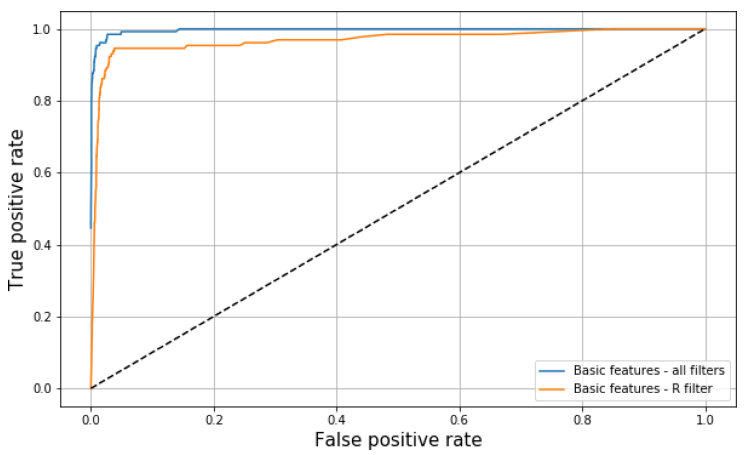
Fig. 9 ROC curve for the efficiency of the classification using only base features with information from the filter r (orange) and information from all the filters (blue). The color figure can be viewed online.
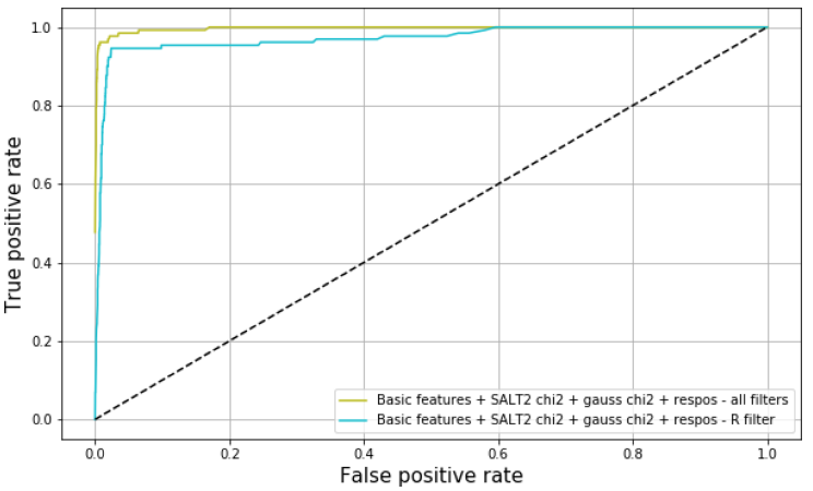
Fig. 10: ROC curve for the efficiency of the classification using all features with information from the filter r (blue) and information from all the filters (green). The color figure can be viewed online.
The importance of all features is shown in Figure 11. The selected features, already studied by [Neira (2020)], proved to be effective. With a 97% precision on other simulated curves and a 89% precision on real supernovae, we can see that the classification with new features was successful, even if the contribution to the efficiency was small. As a matter of fact, even with the possible issues with the flux of simulated supernovae on images, this performance on a real dataset indicates that the algorithm remains flux invariant.
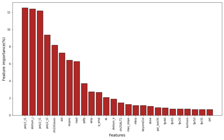
Fig. 11 Feature importance for binary classification of supernovae. The new features (chiSALT, chi2sGauss and respos) have variable non-negligible importance on the classification. The color figure can be viewed online.
When compared with similar classification methods such as the ones proposed by [Pasquet et al.(2019)] and [Muthukrishna et al.(2019)], our results were in line with these works in terms of the AUC values. While we obtained between 0.971 and 0.997 for real data and 0.984 and 0.996 for simulated data and, [Pasquet et al.(2019)] reported between 0.984 and 0.996 for simulated and real data in three different datasets similar to the CFHT ones, whereas [Muthukrishna et al.(2019)] obtained between 0.940 and 0.970, using the PLAsTiCC dataset [The PLAsTiCC team et al.(2018)]. Both works used deep learning and included more source characteristics such as photometric redshift. Further comparisons might be needed using similar datasets; however, we do show that quality improvements along the pipeline and an increase in the amount of information available to find light curves impact positively the results for SNIa detection. We are cautiously optimistic about these results, as they may open new research paths on this subject, in particular, applying these ideas to classify more kinds of supernovae and even other types of transients.
5 Conclusions
In this paper we presented an exploration of possible optimizations for type Ia supernovae detection using the LSSTsp as a base tool. Using this framework, we focused our contributions on studying some changes to the Generation of Difference Images, the Candidate Selection, and the Type Ia Supernova Identification stages.
Our studies demonstrates the importance of fine-tuning a transient detection pipeline through improving the quality of inputs, and consequently, helping the pipeline detect and classify candidates.
We have achieved a relatively high efficiency in the identification of Type Ia Supernovae, and we have showcased how a framework such as the LSSTsp could be used to leverage new studies and open the door to new possibilities exploring the intersection between the application of computational methods, machine learning, and image processing to astronomical surveys.
Overall, we presented different approaches, tweaks, and adaptations to traditional transient detection pipelines. We believe our results are significant enough to justify further exploration in this area.

