nueva página del texto (beta)
 Inglés (pdf)
 Artículo en XML
 Referencias del artículo
 Enviar artículo por email
 Citado por SciELO
  Similares en
SciELO
Similares en
SciELO 
 Permalink
1 Introduction
The rotation pattern observed on two-dimensional velocity maps is the result of the gravitational potential and the mass distribution in a galaxy, together with environmental factors and projection effects [e.g., Rubin & Ford 1970; Binney 2008. In disk-like systems the rotation, or azimuthal velocity, is the dominant velocity component. When this velocity is plotted against the galactocentric distance it describes the rotational curve of a galaxy (e.g. Rubin & Ford 1970; Rubin et al. 1980).
Since early studies of the neutral hydrogen distribution in nearby galaxies, it was possible to obtain resolved velocity fields (e.g., Warner et al. 1973); these Hi velocity maps showed ordered kinematic patterns that, in most cases, could be described by pure circular rotation (e.g., Wright 1971; Begeman 1989; de Blok et al. 2008). Since then, many efforts have been done for recovering rotation curves of galaxies, not only with Hi data, but also with molecular and ionized gas observations. [Begeman(1987), Begeman(1989)] introduced a methodology to extract the rotational velocity curve from two-dimensional (2D) velocity maps based on the so-called tilted rings. This idea became the core of most of the algorithms focused on the determination of the rotation curves of galaxies, for instance the GIPSY task ROTCUR (e.g., Begeman 1987). The tilted ring model assumes that the observed velocity field can be described by pure circular motions with possible variations in the projection angles. From it, several algorithms have been developed to study the kinematic structures of galaxies. On one side are those who uses 3D data-cubes, for instance 3DBarolo (e.g., Di Teodoro & Fraternali 2015), TiRiFiC (e.g., Józsa et al. 2007), GalPak3D (e.g., Bouch´e et al. 2015), KinMSpy (Davis et al. 2013). In a second category are those which work on velocity fields, such as RESWRI (e.g., Schoenmakers 1999), DiskFit (e.g., Sellwood & Spekkens 2015), 2DBAT (e.g., Oh et al. 2018), and KINEMETRY (e.g., Krajnovi´c et al. 2006) among others.
3D algorithms have the advantages of extracting all the information from the datacubes. These methods model the entire datacubes, which allows them to correct for beam smearing effects and also to handle projection effects. However, the inclusion of datacubes usually involves the addition of extra parameters during the fitting process, which in most cases involves longer computing times depending on the dimensions of the datacube and the fitting routine. On the other hand, 2D algorithms work on the projected line of sight velocity (LOSV); for this reason they tend to be faster than 3D methods. If galaxies are not severely affected by spatial resolution effects, (i.e., the observational point spread function, PSF), both methods show consistent results for rotational velocities (e.g., Kamphuis et al. 2015).
Nevertheless, non-circular motions driven by structural components of galaxies (such as spiral arms, bars, bulge), or by angular momentum loss, are not included within the circular rotation assumption (e.g., Kormendy 1983; Lacey & Fall 1985; Wong et al. 2004); nor are those motions induced by internal processes (stellar winds, Hii regions, shocks, outflows). Altogether, and taking into account projection effects, the modeling of non-circular motions is a big challenge. Only a few algorithms take into account deviations of circular motions, among which are: TiRiFiC, ideal for modeling warped disks; DiskFit, suitable to model bar-like and radial flows; and KINEMETRY to model non-circular motions of any order through harmonic decomposition.
For deriving rotational curves, most algorithms adopt frequentist methods that minimize the residuals from a model function and the data, and those parameters that minimize the residuals are chosen for creating the kinematic model that better describes the data. This means that from a frequentist perspective, there is a single set of true parameters that describes the data. Conversely, Bayesian methods assume that model parameters are totally random variables, and each parameter has associated a probability density function. In this way solutions are based on the likelihood of a parameter given the data; that is, on the posterior distribution of the parameters.
These are two different perspectives to estimate the parameters from a model. Rotational curves are often described by several parameters, which makes it a high-dimensional problem, and therefore susceptible to find local solutions. Therefore, it is worth exploring methods that survey the parameter space of kinematic models to derive the best representation of the observed rotation patterns of disk galaxies.
In this paper we introduce XooSuut1(or XS for short). This is a Python tool that implements Bayesian methods for modeling circular and noncircular motions on 2D velocity maps. The name of this tool is a combination of two Mayan words: Xook which means “study” and Suut which means “rotation”.
This paper is organized as follows. In § 2 we describe the different kinematic models included in XookSuut. In § 3 we describe the algorithm, the fitting procedure, and the error estimations. In
2 Kinematic models
In this section we describe the kinematic models included in XookSuut. We start with the simplest model, which is the circular rotation model, then we add a radial term for modeling radial flows. A bisymmetric model is included for describing oval distortions (i.e., bar-driven flows); finally, XookSuut includes a more general harmonic decomposition of the line of sight velocity, for a total of three non-circular rotation models. For constructing these models, XookSuut assumes that galaxies are flat and circular systems and that they are viewed in projection, with a constant position angle (
XookSuut adopts the methodology introduced by DiskFit (e.g., Sellwood & Spekkens 2015) diskfit for creating a two dimensional interpolated map of the referred kinematic models and described in the following sections.
2.1 Circular Model
The simplest model included in XookSuut is the circular rotation model, which is the most frequently adopted for describing the rotation of galaxies. It assumes no other movements than pure circular motions in the plane of the disk and describes the rotation curve of disk galaxies.
Assuming that particles follow circular orbits on the disk, the circular model is given by the projection of the velocity vector
V
t
is the circular rotation or azimuthal velocity and is a function of the galactocentric distance;
2.2 Radial Model
When radial motions are not negligible, the disk circular velocity is described by two components of the velocity vector: the tangential velocity
Comparing with equation 1, the only difference is the addition of the
2.3 Bisymmetric Model
The bisymmetric model describes an oval distortion on the velocity field, such as that produced by stellar bars (e.g., Spekkens & Sellwood 2007; Sellwood & Spekkens 2015), or by a triaxial halo potential. In the presence of an oval distortion particles follow elliptical orbits elongated towards an angle that in general differs from that of the disk position angle (e.g., Spekkens & Sellwood 2007). This kinematic distortion shows a characteristic “S” shape in the projected velocity field that makes the minor and major axes not orthogonal (e.g., Kormendy 1983). Given that this pattern has been mostly observed in the velocity field of barred galaxies, we will refer to the origin of the oval distortion to stellar bars, although it is not necessarily the case, as mentioned before. The model that intends to describe this pattern is called bisymmetric model (e.g., Spekkens & Sellwood 2007) since most of the perturbation is kept in the second order of an harmonic decomposition on the disk plane. The bisymmetric model is described by following the expression:
Note that in this expression both angles are measured on the disk plane. If
where
2.4 Harmonic Decomposition
Similar to the photometric decomposition of galaxy images into light profiles via Fourier expansions, the line of sight (LoS) velocity field of a galaxy can be expressed as a sum of harmonic terms as follows:
where c
m
and s
m
are the harmonic velocities, m is the harmonic number, and
In XooSuut the harmonic model, (equation 6), can be expanded to any harmonic order, although, most of the non-circular motions induced by spiral arms or bars are captured by a third order expansion (e.g., Trachternach et al. 2008).
The harmonic model was first included in the GIPSY task RESWRI I (e.g., Schoenmakers 1999) RESWRI under the assumption of a thin disk. Afterwards the harmonic decomposition was generalized in KINEMETRY (e.g., Krajnovi´c et al. 2006) Kinemetry including not only disks but also triaxial structures. The major difference between RESWRI and XooSuut is the assumption of a flat disk. While RESWRI and KINEMETRY allow varying the disk position angle and inclination during the fitting analysis,
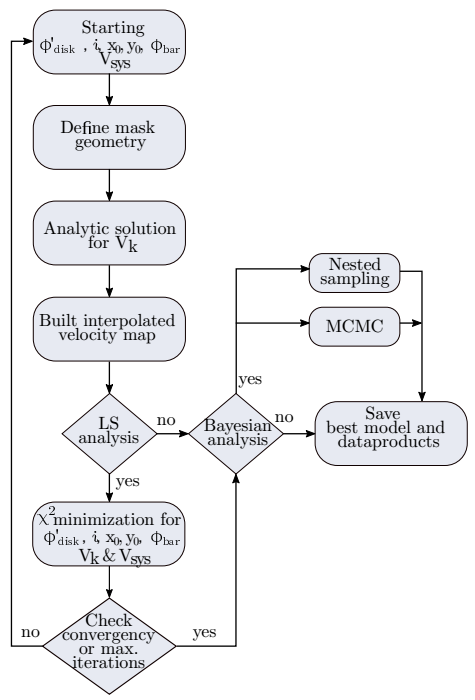
3 The algorithm
XookSuut works on 2D velocity maps, such as those extracted from first moment maps from data-cubes. As others codes that rely on 2D maps for kinematic modelling, XookSuut assumes that the velocity recorded in each pixel is representative of the disk velocity. In this sense, there are a wide variety of methods for representing the velocity field of a galaxy, and many of these depend on the spectral resolution and the signal-to-noise of the data; going from simple first moment maps, to modeling Gaussian profiles in combination with Hermite polynomials to better reproduce the shape of the emission lines (see de Blok et al. 2008; Sellwood et al. 2021, for a revision of different methods).
For XookSuut to obtain confident estimations of the kinematic models, the data should not be strongly affected by the point-spread-function. The PSF contributes to increase the velocity dispersion of the emission-lines and consequently to underestimate the rotation velocities, particularly in the inner gradient of the rotation curve. In such a case, a 3D modeling of the datacubes should be a better approach (e.g., Di Teodoro et al. 2016). Under the previous assumptions the algorithm proceeds in the following way.
Let
The radius of the circle on the disk plane passing through this point is then:
The azimuthal angle on the disk plane
Therefore,
3.1 χ2 Minimization Technique
As we will see in further sections, Bayesian methods like MCMC require to start sampling around the maximum a posteriori, or maximum likelihood, to generate new samples also known as chains; this requires necessarily to find those parameters that minimize the residuals from a given kinematic model and the data. Therefore, in the following we describe the method to solve for each of the different kinematic components of the models, and the constant parameters. The first part corresponds to the analysis adopted in DiskFit (e.g., Spekkens & Sellwood 2007; Sellwood & Spekkens 2015) with minimum changes.
A given set of initial conditions for the geometric parameters defines the projected disk with an elliptical shape on the sky plane. Ideally, the initial conditions for the gaseous disk geometry should be close to that of the stellar disk. This geometry will be the starting configuration for the minimization analysis; then, the field of view is divided into K concentric rings of fixed width that follow the same orientation as before. The maximum length of the ellipse semi-major axis can be easily set-up as described in Appendix A; this will create a 2D mask and only those pixels inside this maximum ellipse will be considered for the analysis. The geometry of this mask will be adapted in subsequent iterations until reaching the orientation that better describes the observed velocity field.
The algorithm will solve for each ring a set of velocities that will depend on the kinematic model considered, namely equations 1-3 or equation 6 . Thus, the number of different velocity components to derive will be K velocities in the circular model (
The velocity map consists of a two-dimensional image of size
Here v is the total number of degrees of freedom (i.e.,
Each kinematic component from
where the super-index t makes reference to the circular rotation component. The radial model requires two different weights for the different kinematic components:
Similarly, the bisymmetric model would require three different weights:
Finally, the harmonic decomposition model will have 2M weights given by:
Note that for M = 1 it reduces to the radial model.
The
where r
k
and r
k+1
are the position of the k
th
and
The first method is to assume that velocities grow linearly from zero to the velocities derived in the first ring (
As
Rearranging this expression we obtain:
The minimization technique from equation 24 was first introduced by Barnes & Sellwood (2003), and subsequently incorporated into DiskFit (Sellwood & Spekkens 2015). Here, equation 24 is generalized for the harmonic decomposition model. The latter expression is a system of linear equations for the
Given a set values for the constant parameters and K rings positioned at r
k
on the disk plane, we can solve for
The minimization procedure in equation 12 is performed by constructing a 2D model from the interpolation weights of equation 21. In each
Rings not proper sampled with data may give absurd values of
To perform the LS analysis in equation 12, XookSuut adopts the Levenberg-Marquardt (LM) algorithm included in the lmfit package (e.g. Newville et al. 2014). This algorithm has the advantage that it is fast, although it is widely known to be susceptible to getting trapped at a local minimum. Note that DiskFit adopts the Powell method since this method only performs evaluation of functions with no derivatives performed.
So far the algorithm adopts an LS method for deriving the best parameters defined by the kinematic models. In the following we use sampling methods to infer the posterior distributions of the parameters.
3.2 Bayesian Analysis
The novelty of XookSuut resides in the estimation of the posterior distribution of the non-circular motions and the model parameters. Given the high-dimension of the models, it is desired to perform a thorough analysis of the prior space to obtain the most likely solutions to the problem for each kinematic model regardless of its complexity. For this purpose we adopt Bayesian inference methods for sampling their posterior distributions. Other packages like 2DBAT and KinMSpy (i.e., Oh et al. 2018; Davis et al. 2013) also use Bayesian approaches for extracting rotational curves of galaxies. The difference is that KinMSpy is able to fit non-circular motions (radial and bisymmetric).
According to Bayes’ theorem, given a set of data
where
with the evidence defined as:
where the integral is computed over all the parameter space defined by the priors,
The final goal of Bayesian inference is to obtain the posterior distribution
Other methods, such as nested sampling (NS, Skilling 2006), are designed to compute the evidence by numerical integration of equation 27, which often makes them computationally more expensive than MCMC methods. This integral is performed from the priors space (or prior volume), and unlike MCMC, does not require an initialization point. Nevertheless, computing the evidence is crucial for model comparison as it represents the degree to which the data are in agreement with the model. Although the main goal of NS is to compute the evidence, the posterior distribution is obtained as a by-product; because of that, NS methods are becoming popular for the inference of parameters in astronomy (see Ashton et al. 2022, for a thorough description of the method).
One of the advantages of nested sampling with respect to MCMC methods is regarding the convergence criteria. There is no defined convergence criteria among MCMC algorithms, although some of them are based on the number of independent samples in the chains, the so-called integrated autocorrelation time (IAT); however this is often evaluated a posteriori. If the whole chain contains between 10-50 times the IAT, then it is a good indicator that chains are converging (Foreman-Mackey et al. 2013; Karamanis et al. 2021). In contrast, in nested sampling the stopping evaluation criterion is well defined, since sampling stops after the whole prior space has been integrated.
A detailed discussion of these two sampling methods is, however, beyond the scope of this paper. Following we show the implementation of MCMC and nested sampling methods for the parameter extraction of the kinematic models presented in Sec. 2.
3.2.1 Likelihood and Priors
Let
The likelihood function is a key term in Bayesian inference, since it will define the shape of the posterior distributions. The most common distribution for the likelihood is Gaussian, but other distributions like Cauchy, T-student, or the absolute value of the residuals are also adopted in the literature (e.g., Di Teodoro & Fraternali 2015; Bouché et al. 2015; Oh et al. 2018). XookSuut adopts the Gaussian distribution as the main likelihood function, although the Cauchy distribution is also included (see Appendix B). The individual likelihood for each data point
and the joint likelihood for the data set is the product of individual likelihoods, in this way
It is easy to recognize from this expression that the summation is the
with N being the number of data points, or pixels, to be considered in the model. We can redefine
The priors are the constrain of our model function and enclose all we know about the data. Uniform or non-informative priors give the same probability to any point within the considered boundaries. This allows the likelihood function to survey the prior space without any preferred direction. XookSuut adopts either uniform or truncated Gaussians (TG), with values shown in Table 1. TG priors are of the form TG(
TABLE 1 Type of priors adopted in XookSuut
| Parameter | Uniform prior | Truncated Gaussiansa |
|---|---|---|
|
|
0 if |
TG( |
| i | 0 if 30 < i < 75 | TG( |
|
|
0 if |
TG( |
| x 0 | 0 if |
TG( |
| y 0 | 0 if |
TG( |
| V sys | 0 | TG( |
| Vk | 0 if |
TG( |
|
|
0 if |
TG(0.1,1,-10,10) |
a Values with hat represent LS results. V k refers to any of the different radial dependent velocities.
In order to infer the posterior distribution of the parameters, XookSuut adopts two well known Python packages for Bayesian analysis; these are the emcee package EMCEE, and DYNESTY (e.g., Foreman-Mackey et al. 2013). EMCEE is a Python implementation of the affine-invariant method for MCMC with automatic chain tuning; while dynesty is a Python implementation of dynamic nested sampling methods. MCMC and NS are two robust sampling techniques to derive posterior distributions in high dimensional likelihood functions, such as the kinematic models described before. Both packages have been extensively applied in astronomy for making Bayesian inference, with particular implementations in cosmology. For a detailed description of these codes we suggest reading their corresponding documentation. Both packages require a set of configurations whose purpose is to guarantee convergence of the sampling procedure. XookSuut is optimized to pass a configuration file to set up EMCEE and DYNESTY. The main setups in these codes are the length of the join-chains and the discarding fraction (burning period) in the case of MCMC, and the integration limit for NS. For both packages, XookSuut adapts the likelihood functions and priors to make it compatible with MCMC or NS methods.
As mentioned before, MCMC samplers like EMCEE sample from the likelihood; therefore the chains need to be initialized at some position, for which XookSuut chooses a random region around the maximum likelihood. For MCMC samplers the joint posterior distribution is estimated up to a normalization constant, here adopted equal to 1 (or zero in ln). For running dynesty XookSuut transform the priors from Table into a unit cube, in such a way that all parameters vary from 0 to 1 and they are re-scaled at the end of the sampling process.
Finally, representative values of the parameters are taken as the 50% percentile of the marginalized distributions. The uncertainty in the parameters is addressed in the following section.
Although emcee makes use of frequentist methods for starting the sampling process, this could be suppressed if relatively good initial positions of the disk geometry are given. On the other hand, dynesty does not require at all the LS initialization as the numerical integration is performed over the prior space.
3.2.2 Error Estimation
The true uncertainty in rotational velocities is known to be underestimated with standard least squares minimization techniques and even with MCMC methods (e.g., de Blok et al. 2008; Oh et al. 2018). Errors estimated with these methods are usually of the order of the turbulence of the ISM (a few km s-1 ) and do not represent the systematic errors. Some works adopt the mean dispersion per ring as a measure of the uncertainty in the rotation curve. However, when non-circular components are added to the model, this assumption is no longer valid since each ring may contain multiple kinematic components.
Additionally, XookSuut also implements a bootstrap analysis for error estimation. Our procedure differs from the one described by [Sellwood S chez(2010)], as explained below. The residuals from the best 2D interpolated model are used to generate new samples. Instead of shuffling residuals at random locations on the disk, K rings of width
In general, we find that the estimated uncertainties of the parameters increase in the following order: Bayesian methods > bootstraps > LS, with computational cost increasing in the same direction.
4 Testing XookSuut
We now proceed to evaluate XookSuut in a series of simulated velocity maps and real velocity fields.
4.1 Toy Model Example
As an example of its use, we run XookSuut on a simulated velocity map. This is the velocity field of a galaxy at 31.4 Mpc with a 32 optical radius. We model a velocity field with an oval distortion described by equation 3. For the rotation curve we adopt the parameterization from Bertola et al. (1991).. The non-circular motions were modeled using the Gamma probability density function; Gamma(2,3.5) for describing the
We started XookSuut by assigning random values to each of the constant parameters, except for
On the other hand, nested sampling only requires the prior information, for which we adopted the uniform priors from Table 1. No initial LS was performed for this case. We stopped the sampling procedure only when the remaining evidence to be integrated was
We test all the different kinematic models, i.e., circular, radial, bisymmetric models and we arbitrarily expand the harmonic series up to M = 3. MCMC and NS derive the posterior distribution for each variable of the kinematic model; thus, we can take advantage of corner plots to represent their marginalized distributions and explore possible correlations between parameters. The median values and
TABLE 2 Best fit parameters for the toy model example
| Model | Method |
|
Δi |
|
|
|
|
RMS | BIC |
| (°) | (°) | (pix) | (pix) | (km s-1 ) | (°) | (km s-1) | |||
| circular | LM | -1.1 ± 0.1 | -0.4 ± 0.1 | 0.0 ± 0.0 | 0.1 ± 0.0 | -0.0 ± 0.2 | 8.5 | 4.5 | |
| MCMC | -1.1 ± 0.1 | -0.1 ± 0.3 | 0.0 ± 0.1 | 0.1 ± 0.1 | -0.0 ± 0.2 | 9.3 | 4.5 | ||
| NS | -1.1 ± 0.1 | -0.1 ± 0.3 | 0.0 ± 0.1 | 0.1 ± 0.1 | -0.0 ± 0.2 | 9.3 | 4.5 | ||
| radial | LM | -0.1 ± 0.1 | -0.2 ± 0.2 | 0.0 ± 0.0 | 0.1 ± 0.0 | 0.0 ± 0.2 | 9.3 | 4.4 | |
| MCMC | -0.1 ± 0.1 | 0.1 ± 0.3 | 0.0 ± 0.1 | 0.1 ± 0.1 | -0.0 ± 0.2 | 8.5 | 4.4 | ||
| NS | -0.1 ± 0.1 | 0.0 ± 0.3 | 0.0 ± 0.1 | 0.1 ± 0.1 | -0.0 ± 0.2 | 8.5 | 4.4 | ||
| bisymmetric | LM | 0.0 ± 0.1 | 0.1 ± 0.2 | 0.0 ± 0.0 | 0.1 ± 0.0 | -0.0 ± 0.2 | 3.8 ± 8.0 | 8.5 | 4.4 |
| MCMC | 0.0 ± 0.2 | 0.1 ± 0.3 | 0.0 ± 0.1 | 0.1 ± 0.1 | -0.0 ± 0.2 | 3.7 ± 7.8 | 8.5 | 4.4 | |
| NS | 0.0 ± 0.2 | 0.1 ± 0.3 | 0.0 ± 0.1 | 0.1 ± 0.1 | -0.0 ± 0.2 | 3.6 ± 8.2 | 8.5 | 4.4 | |
| harmonic | LM | -0.1 ± 0.1 | -0.0 ± 0.3 | 0.0 ± 0.0 | 0.1 ± 0.0 | -0.0 ± 0.2 | 8.5 | 4.4 | |
| MCMC | -0.1 ± 0.1 | 0.0 ± 0.3 | 0.0 ± 0.1 | 0.1 ± 0.1 | -0.0 ± 0.2 | 8.5 | 4.4 | ||
| NS | -0.1 ± 0.1 | 0.0 ± 0.3 | 0.0 ± 0.1 | 0.1 ± 0.1 | -0.0 ± 0.2 | 8.5 | 4.4 |
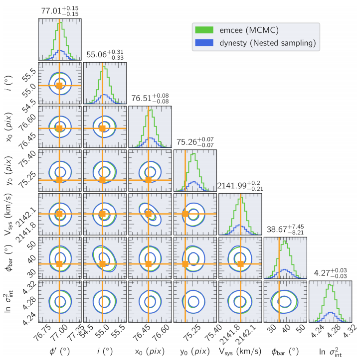
Fig. 2 Marginalized distributions of the parameters describing the bisymmetric model for our toy model described in § 4.1. This corner plot shows only the parameters describing the disk geometry. Contours enclose 68% and 95% of the data. Histograms of individual distributions are shown on top, together with the median values and
MCMC and nested sampling methods converge to the same solutions found by the LS method; this represents a great success for Bayesian methods to derive kinematic parameters from an input velocity map given the large dimension of the likelihood function. We note that the input parameters are recovered in the bisymmetric model, which is not the case for the circular, radial and harmonic, as expected; this is better appreciated in the corner plot from Figure 2. MCMC and nested sampling recover the input parameters within the
The different velocities,
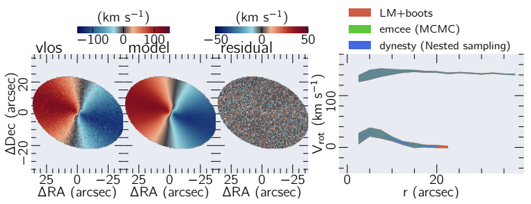
Fig. 3 XookSuut results for the toy model example, for the bisymmetric model case. Figures from left to right: simulated velocity field; best two dimensional interpolated model from MCMC; residual map (input minus output). Overlaid on these maps are iso-velocity contours starting at 0 km s-1 with steps of
Table 2 also shows the root mean square (RMS) for each kinematic model; models including non-circular rotation show a RMS value around 8.5 km s-1 . This leads to the question of which model is the preferred one for describing a particular velocity field. In a statistical sense, when comparing different models one should choose the one with fewer parameters, since more variables in a model often reduce further the RMS, which does not necessarily provide the best physical interpretation of the data. Statistical tests such as the Bayesian information criterion (BIC) penalizes over the variables from the model; BIC is defined in terms of the likelihood (or the chi-square) as,
However, when there is little information about the data, or only the data itself, it is difficult to select a model description of the data based on any information other than statistical tests. Regardless of the statistical method adopted, it is important to have a physical motivation for accepting or rejecting a model; otherwise, erroneous interpretations of the velocity field could arise.
For the toy model example, Table 2 shows that non-circular models have similar BIC values. Even when the harmonic decomposition model seems to perform a good fitting based on the residuals, the physical interpretation of the m = 2 components are meaningless for this example. Thus in a real scenario the radial and bisymmetric model should be compared. The Bayesian evidence for the radial and bisymmetric models results in
4.2 Simulations
We carried out a set of 1000 simulations with different inclination angles ranging from
In Figure 4 we show the results of the analysis in corner plots; the derived values are shown relative to the true ones, namely
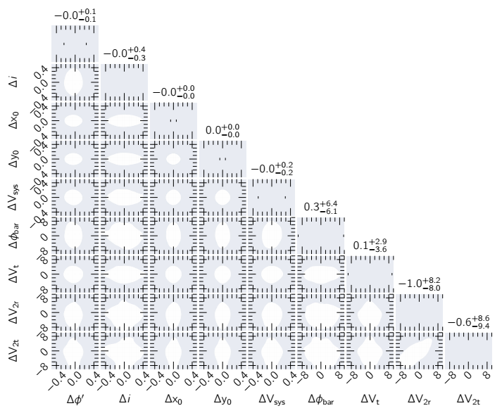
Fig. 4 XookSuut results for the bisymmetric model on 1000 synthetic velocity maps with oval distortions. Values are reported with respect their true value, namely
The final accuracy of the recovered parameters would depend on the details of data themselves (resolution, S/N , spatial coverage etc.). Therefore, ad-hoc simulations are encouraged.
4.3 NGC 7321
We proceed to evaluate XookSuut over the velocity field of a galaxy hosting a stellar bar. For this purpose we adopt the galaxy NGC 7321 observed as part of the CALIFA galaxy survey (e.g., Sánchez et al. 2012). This object has been previously analyzed by Holmes et al. (2015) using DiskFit. The H
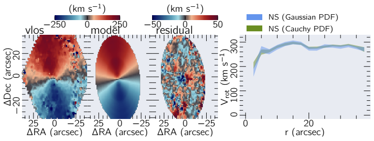
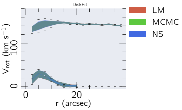
Figure 5 shows the marginalized distributions of the constant parameters. From the 1D histograms we obtain
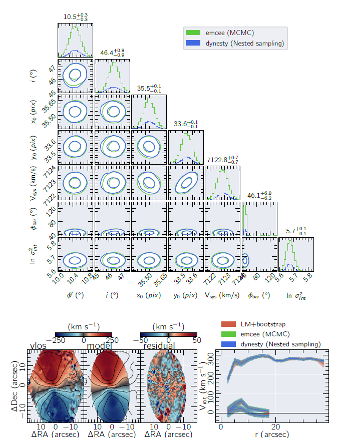
Fig. 5 XookSuut results for NGC 7321 for the bisymmetric model. Top figure shows the marginalized distribution for the constant parameters with MCMC methods in green colors and NS in blue. As in Figure 2, the quoted values on top the histograms represent the median and 2
TABLE 3 XookSuut bisymmetric results for NGC 7321
| Method |
|
i | x0 | y 0 | Vsys |
|
| (°) | (°) | (pixels) | (pixels) | (km s-1 ) | (°) | |
| LS+bootstraps | 11 ± 1 | 46 ± 1 | 35.5 ± 0.0 | 33.6 ± 0.0 | 7123 ± 1 | 46 ± 4 |
| NS | 11 ± 0 | 46 ± 1 | 35.5 ± 0.1 | 33.6 ± 0.1 | 7123 ± 1 | 46 ± 6 |
| MCMC | 11 ± 0 | 46 ± 1 | 35.5 ± 0.1 | 33.6 ± 0.1 | 7123 ± 1 | 46 ± 7 |
| DiskFit* | 12 ± 1 | 46 ± 1 | ... | ... | 7123 ± 3 | 47 ± 6 |
*Results from Holmes et al. (2015). Errors in Holmes et al. (2015) represent
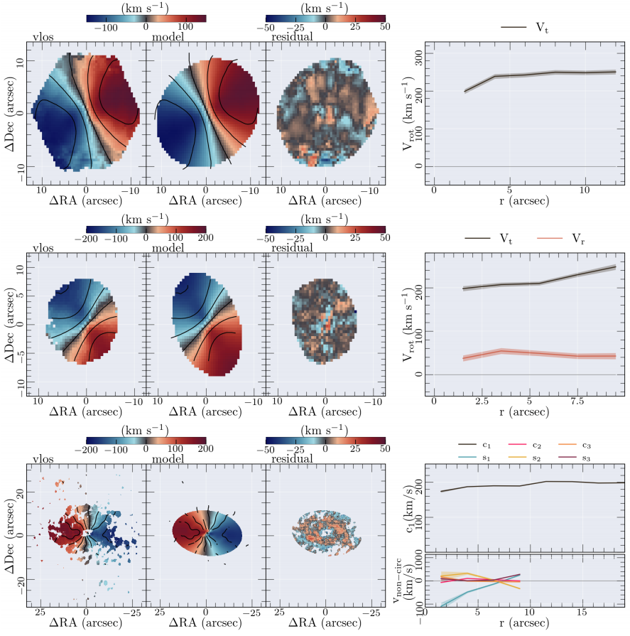
In Appendix D we show the implementation of XookSuut on other data with different instrumental configurations.
5 Discussion
Our simulations and toy example show that sampling methods are able to produce results similar to those obtained with frequentist methods based on the
Bayesian methods, i.e., MCMC and NS, provide the largest uncertainties on the parameters compared to the two other techniques. The major disadvantage is the computational cost needed to sample the posterior distributions. For the toy model example presented, the execution times on an 8 core machine are
If Bayesian methods and LS+bootstrap provide similar solutions for the parameters, then in principle one could choose either of the two methods to quote the uncertainties. However, the most interesting cases are when Bayesian methods differ from the frequentist ones.
6 Conclusions
We have presented a tool for the kinematic study of circular and non-circular motions of galaxies with resolved velocity maps. This tool named XookSuut (or XS for short), is an adaptation of the DiskFit algorithm, designed to perform Bayesian inference on parameters describing circular rotation, radial flows, bisymmetric motions and an arbitrary harmonic decomposition of the LoS velocities. XookSuut implements robust Bayesian sampling methods to obtain the posterior distribution of the kinematic parameters. In this way, the “best-fit” values, and their uncertainties are obtained from the marginalized distributions, unlike frequentist methods where best values are obtained at a single point from the likelihood function. XookSuut adopts Markov Chain Monte Carlo methods and dynamic nested sampling to sample the posterior distributions. In particular, XookSuut makes use of the emcee and dynesty packages developed to perform Bayesian inference.
XookSuut is a free access code written in Python language. The details about running the code, as well as the required inputs and the outputs are described in Appendix A.
XookSuut is suitable to use on velocity maps not strongly affected by spatial resolution effects, i.e., when the PSF FWHM is smaller than the size of structural components of disk galaxies, such as stellar bars. In addition, disk inclination should range from 30° < i < 70°. The fundamental assumption of the code is that galaxies are flat systems observed in projection on the sky with a constant inclination angle, constant disk position angle and fixed kinematic center. This makes XookSuut suitable for studying the kinematics of galaxies within dynamical equilibrium, but not for highly perturbed disks.
Applying XookSuut over a set of simulated maps with oval distortions we showed that Bayesian methods are able to recover the input parameters despite the high dimension of the likelihood function. True parameters are recovered within
Regarding the uncertainty of the parameters, Bayesian methods provide the largest uncertainties compared with resampling methods like bootstrap. However, the computational cost for sampling the joint posterior distribution is in general more expensive than, for instance 1k bootstraps. Fortunately, a fraction of time can be saved when these methods are run in parallel.
We also tested XookSuut on velocity maps from different galaxy surveys. Despite the instrumental differences in these data, XookSuut is able to build kinematic models of circular and non-circular motions.
Finally, XookSuut is ideal for running on individual objects, or in galaxy samples since it is easy to systematize for use in large data sets. XookSuut is a free access code available at the following link https://github.com/CarlosCoba/XookSuut-code.