4.1. Disc and Halo Models

In this work, we use the method described by ^{Sofue (2012)}, where the total rotation velocity at radius 𝑅 is defined as:

where 𝑉_𝑡 is the total rotation velocity and 𝑉_𝑏,𝑉_𝑑,𝑉_ℎ,𝑉_𝐻𝐼 are the rotation velocity components for the bulge, disc, DM halo and HI disc, respectively. For the present study, since our sample is composed of late spiral and irregular galaxies, we will consider the velocity contribution of a bulge component as negligible.

The stellar disc velocity component, 𝑉_𝑑, was determined with the analytical expression obtained from the Poisson equation for a thin disc following an exponential surface density profile and a constant M/Lalong the radius (^{Freeman 1970}; ^{Binney & Tremaine 1987}).

where 𝑀 _𝑑 is the total stellar disc mass, 𝑎 _𝑑 the exponential scale radius and 𝐷 (𝑋) is defined as:

being 𝐼 _𝑖 y 𝐾 _𝑖 the modified Bessel functions and X =Rαd . The two free parameters are the total stellar disc mass, 𝑀 _𝑑 , and the exponential scale radius, 𝑎 _𝑑 . In the present investigation, the DM halo was modelled assuming three different density profiles: Navarro-Frenk-White (hereafter, NFW) (^{Navarro et al. 1997}), pseudo-isothermal (ISO) (^{Kent 1986}), and Burkert-type (BURK) (^{Burkert 1995}). They are described as:

where 𝜌 ₀ is the core density and ℎ is the scale length of the DM halo. Considering spherical symmetry, the total halo mass is obtained by integrating along the radius, giving the following expressions for the NFW, ISO and BURK profiles, respectively:

The rotation velocity component for the dark matter halo at radius 𝑅 is:

DM density profiles are often expressed in terms of the rotation velocity at the virial radius, 𝑉 ₂₀₀, and the concentration parameter, 𝑐, defined as:

where 𝑅 ₂₀₀ is the radius of a spherical halo with a mass equal to 𝑀 ₂₀₀ and the virial mass 𝑀 ₂₀₀ is defined as the total mass contained within a sphere whose mean density equals 200 times the critical density of the Universe (𝜌 _𝑐 ) at 𝑧 = 0

We have considered a Hubble constant value of 𝐻 ₀ = 73 𝑘𝑚 𝑠 ⁻¹ 𝑀𝑝𝑐 ⁻¹ (^{Riess et al. 2022}) throughout this investigation. This value is the same as the one assumed in the published fits used as comparison (^{Li et al. 2020}).

4.2. HI Disc Velocity Component

Since all the elements in our sample are classified as late-type galaxies (mostly Sm and Irr), it should be necessary to take into account the dynamical effects of a separate HI disc component because such galaxies tend to have an important fraction of their total baryonic mass in the form of HI (^{Roberts 1962}; ^{Huchtmeier & Richter 1989}; ^{Korsagaetal.2019}). In this work, the HI disc velocity component is obtained from the SPARC database HI mass model for each galaxy. This component tis calculated with the ^{Casertano (1983)} formula. In this investigation, in order to isolate the contributions of the stellar disc and DM halo, the HI disc velocity component for each point in the RC is subtracted from the observed rotation velocity using the following expression:

where 𝑉 _𝑜𝑏𝑠 is the observed rotation velocity , 𝑉 _𝐻𝐼 the HI disc velocity component and 𝑉 _{𝑐𝑜𝑟𝑟} the corrected velocity. This latter component is then inserted in the fitting algorithm and analysed.

4.3. Photometry and (𝑀/𝐿) _★ Ratio

In all the problems that involve the fitting of observational data using a certain theoretical model it is important to select a suitable set of constraints to ensure that our algorithm does not give unrealistic results. One important constraint in RC analysis is the surface brightness photometry (^{Katz et al. 2017}; ^{Korsaga et al. 2019}; ^{Li et al. 2020}). The surface brightness profile of the galaxy provides information about how the stars are distributed throughout the disc. In recent years, many studies have shown that near-infrared (NIR) surface photometry can be used as an excellent stellar disc mass tracer, since these bands are less susceptible to systematic uncertainties caused by dust emission that afflict the optical bands (^{Kennicutt et al. 2003}; ^{Leroy et al. 2008}; ^{Meidt et al. 2014}). Another reason is that most of the stellar disc total mass is composed of low-mass stars, whose main emission is at NIR bands (^{Kroupa & Jerabkova 2021}). This is seen as a low dispersion on the (𝑀/𝐿)-color correlation at NIR bands compared to the optical bands (^{Bell & de Jong 2001}). In this work, we used the exponential disc scale length (𝑎 _𝑑 ) and the 3.6 𝜇m total luminosity (LT3.6μm), extracted from the SPARC database (Table 1). It is important to note that, although the thin disk model (^{Freeman 1970}; ^{Binney & Tremaine 1987}) represents a simplification with respect to models used in other studies, it has the advantage of only depending on two photometric parameters (𝐿 _𝑇 , 𝑎 _𝑑 ) to estimate the stellar disk contribution, instead of requiring a complete luminosity profile obtained with high spatial resolution observations (^{Casertano 1983}). In the case of low-mass galaxies, the exponential profile is usually a good approximation for a large interval of radii (^{Lelli et al. 2016}b). However, it is common to find small deviations on the disc caused by secondary structures, such as bars or spiral arms.

Another important constraint in our model is the (𝑀/𝐿) _★ ratio for the stellar disc. As mentioned in the Introduction, the uncertainty in this parameter is mainly responsible for the disc-halo degeneracy. A way to counter this degeneracy is by considering the maximal disc hypothesis, where the contribution of the disc mass to the RC is considered to be as large as the RC itself allows it. Qualitatively, it is defined as a disc whose contribution to the total potential exceeds the contribution of the dark matter halo in the inner regions. However, in recent years evidence was found suggesting that the application of the maximum disc hypothesis usually resulted in (𝑀/𝐿) _★ values that were too high compared to those predicted by the stellar population synthesis (SPS) models (^{McGaugh & Schombert 2014}; ^{Schombert & McGaugh 2014}). This effect is more noticeable in late type galaxies (Sc, Sd, Irr), where the contribution of a bulge is small or nonexistent. Thus, when a plausible range for (𝑀/𝐿) _★ is considered, the resulting fits show DM halos whose contributions to the total rotation velocity are dominant at all radii. The discs that show this property are classified as submaximal (^{Sackett 1997}).

For this first implementation and testing of our procedure, we decided to fix the (𝑀/𝐿) _★ ratio instead of considering it as a free parameter. This was done in order to avoid adding another free parameter to the algorithm, hampering the interpretation of our results. We fixed this ratio at (𝑀/𝐿) _★ = 0.5, constant along the disc, which many studies have converged to take as the fiducial valueat 3.6 𝜇m (^{McGaugh & Schombert 2014}; ^{Schombert & McGaugh 2014};^{Lellietal.2016a}), consistent with the results of stellar population synthesis (SPS) models (^{Bruzual & Charlot 2003}; ^{Meidt et al. 2014}).

4.4. AGA Selection Criterion, the χR2 Function

As we briefly mentioned in the Introduction, in the present work we use the χR2 function as the selection criterion for AGA, which is defined as:

where 𝑁 is the number of RC data points, 𝑃 the number of free parameters, Viobs the observed rotation velocity, Vit the calculated total rotation velocity and 𝜎 _𝑖 the observational uncertainties. After establishing the photometry constraints, the remaining free parameters are the ones corresponding to the DM halo (𝜌 ₀ and ℎ), thus 𝑃 = 2.

4.5. Uncertainty Estimation

In order to estimate the uncertainty range of our results, we use the methodology described in the AGA main paper (^{Cantó et al. 2009}), based in the generation of synthetic data sets. The process is quite simple: for each data point of the measured curve, a random data point is generated inside the observational velocity uncertainty interval 2𝜎. The procedure is repeated until a set of synthetic RCs is obtained. These synthetic curves serve as statistical equivalents on the uncertainty estimation. Each one is treated and analysed in the same way as the measured RCs. The formula used for the generation of synthetic RCs is:

where 𝑉 ^′ (𝑅) is the synthetic rotation velocity value, 𝑉 _𝑜𝑏𝑠 (𝑅) the measured rotation velocity, 𝜎 the observational error and 𝜉 is a random variable in the interval [0, 1]. In the present work, the uncertainties were estimated using sets with an average of 6 synthetic RCs per galaxy. This number was chosen after some tests designed to find the best compromise between time and accuracy. The uncertainties are defined as the standard deviation of the parameter distribution for the synthetic data set.

4.6. Python Subroutine

Adapting AGA to our procedure required to implement some modifications in the code. As mentioned in section 4, the stellar disc contribution is calculated from equation (2), which contains the first and second order modified Bessel functions. The language in which AGA is compiled (FORTRAN90) does not support these functions implicitly, so it was necessary to add them as an external module. These functions were adapted from the FORTRAN special function package, SPECFUN (^{Cody 1993}). Individual tests were performed for each function to ensure they worked correctly.

The fitting procedure was compiled as a Python subroutine, whose main purpose was to provide AGA with all the information needed from a set of machine-readable tables containing the SPARC data for each galaxy in the sample. These data consisted of the measured RC, the disc exponential scale length (𝑎 _𝑑 ), the galaxy total luminosity at 3.6 𝜇m (L⨀3.6μm) and the HI velocity component. Once a fit was obtained for the specified RC, the subroutine then estimated the corresponding 𝑐, 𝑉 ₂₀₀, 𝑀 ₂₀₀ and 𝑅 ₂₀₀ values by using the numerical solver included in the SYMPY package (^{Meurer et al. 2017}). In order to guarantee a good coverage of the parameter space, we established a set of loose constraints for our fitting variables. In the case of the DM profile core density, 𝜌 ₀, we set a range between 0 ≤ 𝜌 ₀ ≤ 1 𝑀 _⊙ pc⁻³, while the scale parameter ℎ could vary between 0 ≤ ℎ ≤ 100 kpc. The typical values of 𝜌 ₀ and ℎ tend to be of the order of 𝜌 ₀ ≈ 10⁻² 𝑀 _⊙ pc⁻³ and ℎ ≈ 10³ − 10⁴ pc (^{Sofue 2012}, ²⁰¹³).

Each AGA run consisted of 150 generations, containing 1000 individual points in the parameter space (200 parent + 800 offspring), with a box size factor of 0.5 between generations. The box size factor reduces the parameter-space volume from which new points can be generated around each individual between one generation and the next. Every AGA run starts with a box size spanning the full specified parameter range. The result is then stored and used as a starting point for the next run. This procedure may seem redundant at first, but it is important to note that for each run, the sizes of the sampling boxes are reset to their initial values, so each run starts searching for the solution using boxes of the same size as the ones used in the first run, but centered on improved initial values (^{Canto et al. 2009}). This enhances the accuracy of´ the algorithm and reduces the probability of converging on a local minimum. Finally, after 6 consecutive runs, the results are stored as the best-fit parameters.

5.1. Comparison with Previous Results

Figures 1 and 2 compare our obtained best-fit parameter values against their corresponding values found in the literature (^{Li et al. 2020}) assuming each DM density profile for the parameters 𝑐 and𝑉 ₂₀₀, respectively. A qualitative analysis shows that most galaxies in these diagrams lie near the red 𝑦 = 𝑥 line, within uncertainties, implying a great degree of consistency between studies. However, some deviations were found (e.g. Figure 2, top), which will be addressed below.

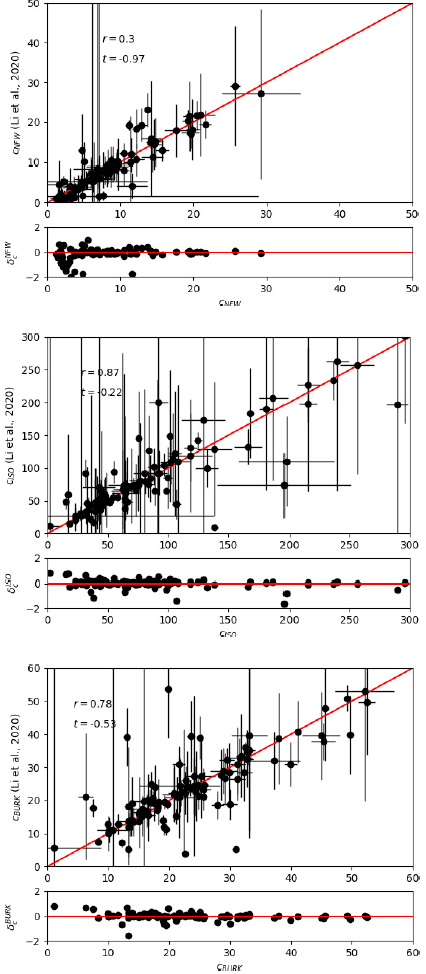
Fig. 1 Comparison diagrams of the best-fit 𝑐 values obtained with our procedure against their corresponding published fits in the SPARC database (^{Li et al. 2020}). The 𝑦 = 𝑥 line is indicated in red. The corresponding residual graphs, described in terms of the deviation parameter 𝛿 _𝑐 (Equation 17) are located below each comparison diagram. On all DM profiles, most galaxies in our sample (≳ 90%) lie within 𝛿 _𝑐 ≤ 1. The color figure can be viewed online. 

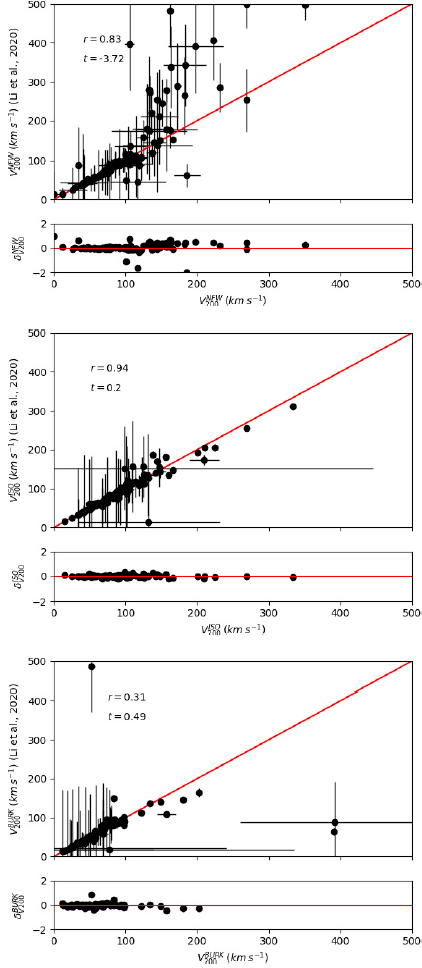
Fig. 2 Comparison diagrams of the best-fit𝑉200 values obtained with our procedure against their corresponding published fits in the SPARC database (^{Li et al. 2020}). The 𝑦 = 𝑥 line is indicated in red. The corresponding residual graphs, described in terms of the deviation parameter 𝛿 _𝑉200 (equation 18) are located below each comparison diagram. On all DM profiles, most galaxies in our sample (≳ 90%) lie within 𝛿 _𝑉200 ≤ 1. The color figure can be viewed online. 

In order to verify in a quantitative manner if our results are consistent with those found in the literature, we compared our obtained best-fit𝑐 and𝑉 ₂₀₀ samples against their corresponding published values through a set of paired 𝑡tests. According to these tests, for a sample size of 100 galaxies with a 95% confidence level, the critical 𝑡 value, 𝑇 (from which we can reject the same-mean hypothesis) is equal to 1.98. If the absolute values of 𝑡 _𝑐 or 𝑡 _𝑉200 are higher than𝑇, we can consider that the difference between the means of our compared samples is statistically significant. The 𝑡-test results, along with their corresponding Pearson correlation values for the parameters 𝑐 (𝑟 _𝑐 ) and 𝑉 ₂₀₀ (𝑟 _𝑉200 ) are condensed in Table 2.

The 𝑡-test analysis shows that our fits pass the equal mean hypothesis in 5 out of the 6 possible tests (2 fit parameters, 3 DM profiles). The only 𝑡-test that did not pass corresponds to the comparison between our obtained vs the published V200NFW samples. This is seen in the V200NFW comparison diagram (Figure 2, top) as a divergence from the 𝑦 = 𝑥 line at V200NFW ≳ 200 km s⁻¹ . It is interesting to note that most of the galaxies that deviate from the y = x line show ℎ values that lie near the upper limit imposed for our procedure (ℎ ≈ 100 kpc), indicating that the global minimum probably did not fall inside our specified ℎ range. In order to explore this, several runs were performed assuming different upper range values for ℎ. We found that, although the χR2 global minimum was reached, the resulting parameter values would not be physical (i.e. 𝑉 ₂₀₀ > 500 km s−1) (^{Li et al. 2020}). This behaviour was found exclusively when a NFW profile was considered.

Along with the 𝑡-tests, to quantify the deviation between the obtained and the published parameter values for each individual galaxy, we define a deviation parameter (𝛿 _𝑐 and 𝛿 _𝑉200 for 𝑐 and 𝑉 ₂₀₀, respectively) by using the following expressions:

where 𝑐 ^𝑏𝑖𝑏 and V200bib are the published 𝑐 and 𝑉 ₂₀₀ values from SPARC, respectively. The number of galaxies in our sample with 𝛿 _𝑐 and 𝛿 _𝑉200 below different thresholds is described in Table 3.

Table 3 shows that in the case of the ISO and BURK profiles the fraction of galaxies in our sample with |𝛿 _𝑐 | ^, |𝛿 _𝑉200 | ≤ 1 is 95% and 94%, respectively, while the NFW profile only reached 85%. These results indicate that the core-type profiles, such as ISO and BURK, are closer to the respective published values than those obtained assuming a NFW profile.

Regarding the Pearson correlation (𝑟 _𝑐 ,𝑟 _𝑉200 ) between datasets (Table 2), high values (𝑟 _𝑐 ,𝑟 _𝑉200 ≈ 0.8 − 0.94) are observed in 4 out of the 6 comparison diagrams (Figures 1 and 2), implying a good compliance of our results with the literature. In contrast, two of these cases show low correlation values (𝑟 _𝑐 ,𝑟 _𝑉200 ≈ 0.3), specifically in the 𝑐 _𝑁𝐹𝑊 comparison diagram (Figure 1, top) and the V200BURK diagram (Figure 2, bottom). These low values are consequence of a handful of outlying galaxies with exceptionally high 𝛿 _𝑐 or 𝛿 _𝑉200 : one in the 𝑐 _𝑁𝐹𝑊 diagram (F571-8) and three in the V200BURK diagram (NGC0247, UGC11557 and D631-7). The main cause for the observed inconsistencies in these galaxies may be attributed to multiple factors, e.g. a divergence from a pure exponential profile in the stellar disk produced by secondary features (i.e. a bar or bulge), or artifacts produced by the use of different numerical solver routines between studies. Without taking into account the outlying galaxies, the correlation values between the samples are 𝑟 _𝑐 = 0.93 and 𝑟 _𝑉200 = 0.92 for the 𝑐 _𝑁𝐹𝑊 and V200BURK comparison diagrams, respectively. It is important to emphasize that these galaxies represent a small fraction of the total sample. Most of the galaxies analysed with our procedure (≳ 85%), show consistency with the literature. The influence of other factors, such as the assumed stellar disc (M/L)* value and the consideration of a separate HI disc component in the resulting mass profile fits, will be explored in a future work.

5.2. Comparison Between Our Results

A comparison of our best-fit parameter samples assuming different DM models serves as an internal consistency check for our procedure. Figures 3 and 4 show all the comparison diagrams (ISO vs NFW, BURK vs NFW and BURK vs ISO) between our best-fit parameter samples 𝑐 and 𝑉 ₂₀₀, respectively. A qualitative analysis shows that all comparison diagrams display a positive trend, with varying degrees of dispersion. In the case of the 𝑐 parameter (Figure 3), we found high correlation values (𝑟 ≈ 0.9) in all comparisons, displaying a nearly linear trend. For the case of 𝑉 ₂₀₀, the diagrams show lower correlation values (0.43 ≤ 𝑟 ≤ 0.71) and in general, a greater dispersion. This could imply a difference in the sensibility between fitting parameters. From this comparison, we conclude that in general our results show consistency between different models.

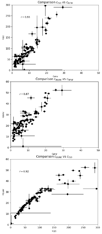
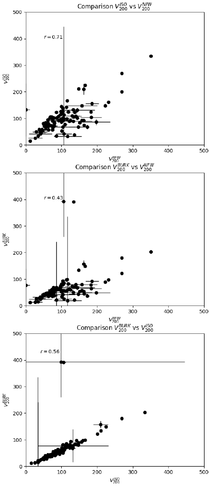
Fig. 3 Comparison diagrams between our obtained best-fit 𝑐 samples assuming different DM profiles. 

Fig. 4 Comparison diagrams between our obtained best-fit𝑉200 samples assuming different DM profiles.

REFERENCES

Abdurro’uf Accetta, K., Aerts, C., et al. 2022, ApJS, 259, 35, https://doi.org/10.3847/1538-4365/ac4414 [ Links ]
Aniyan, S., Freeman, K., Arnaboldi, M., et al. 2018, MNARAS, 476, 1909, https://doi.org/10.1093/mnras/sty310 [ Links ]
Bell, E. F. & de Jong, R. S. 2001, ApJ, 550, 212, https://doi.org/10.1086/319728 [ Links ]
Binney, J. & Tremaine, S. 1987, Galactic Dynamics, (Pincenton, NJ: PUP) [ Links ]
Blais-Ouellette, S., Amram, P., & Carignan, C. 2001, AJ, 121, 1952, https://doi.org/10.1086/319944 [ Links ]
Bosma, A. 1978, The distribution and kinematics of neutral hydrogen in spiral galaxies of various morphological types, PhD. Thesis, Groningen Univ. [ Links ]
______. 1981, AJ, 86, 1825, https://doi.org/10. 1086/113063 [ Links ]
Bruzual, G. & Charlot, S. 2003, MNRAS, 344, 1000, https://doi.org/10.1046/j.1365-8711.2003.06897.x [ Links ]
Burkert, A. 1995, AJ, 447, 25, https://doi.org/10.1086/ 309560 [ Links ]
Cantó, J., Curiel, S., & Martínez-Gómez, E. 2009, A&A, 501, 1259, https://doi.org/10.1051/0004-6361/ 200911740 [ Links ]
Carignan, C. & Freeman, K. C. 1985, ApJ, 294, 494, https://doi.org/10.1086/163316 [ Links ]
Casertano, S. 1983, MNRAS, 203, 735, https://doi.org/10.1093/MNRAS/203.3.735 [ Links ]
Cody, W.J. 1993, ACM Transactions on Mathematical Software, 19, 22, https://doi.org/10.1145/151271.151273 [ Links ]
Curiel, S., Cantó, J., Georgiev, L., Chávez, C., & Poveda, A. 2011, A&A, 525, 78, https://doi.org/10.1051/0004-6361/201015693 [ Links ]
de Blok, W. J. G. 2010, AdAsT, 2010, https://doi.org/10.1155/2010/789293 [ Links ]
Freeman, K. C. 1970, ApJ, 160, 811, https://doi.org/10.1086/150474 [ Links ]
Holland, J. H. et al. 1992, Adaptation in Natural and Artificial Systems. An Introductory Analysis with Applications to Biology, Control, and Artificial Intelligence, (Cambridge, MA: MIT Press) [ Links ]
Huchtmeier, W. & Richter, O.-G. 1989, A&A, 210, 1 [ Links ]
Katz, H., Lelli, F., McGaugh, S. S., et al. 2017, MNRAS, 466, 1648, https://doi.org/10.1093/mnras/stw3101 [ Links ]
Kennicutt, R. C. Jr., Armus, L., Bendo, G., et al. 2003, PASP, 115, 928, https://doi.org/10.1086/376941 [ Links ]
Kent, S. M. 1986, AJ, 91, 1301, https://doi.org/10.1086/114106 [ Links ]
Korsaga, M., Epinat, B., Amram, P., et al. 2019, MNRAS, 490, 2977, https://doi.org/10.1093/mnras/stz2678 [ Links ]
Kroupa, P. & Jerabkova, T. 2021, arXiv:2112.10788, https: //doi.org/10.48550/arXiv.2112.10788 [ Links ]
Kuzio de Naray, R., McGaugh, S. S., & de Blok, W. J. G. 2008, ApJ, 676, 920, https://doi.org/10.1086/527543 [ Links ]
Lelli, F., McGaugh, S. S., & Schombert, J. M. 2016a, ApJ, 816, 14, https://doi.org/10.3847/2041-8205/816/1/L14 [ Links ]
______. 2016b, AJ, 152, 157, https://doi.org/10. 3847/0004-6256/152/6/157 [ Links ]
Leroy, A. K., Walter, F., Brinks, E., et al. 2008, AJ, 136, 2782, https://doi.org/10.1088/0004-6256/136/6/2782 [ Links ]
Li, P., Lelli, F., McGaugh, S., & Schombert, J. 2020, ApJs, 247, 31, https://doi.org/10.3847/1538-4365/ab700e [ Links ]
Marchesini, D., D’Onghia, E., Chincarini, G., et al. 2002, ApJ. 575, 801, https://doi.org/10.1086/341475 [ Links ]
McGaugh, S. S., Rubin, V. C., & De Blok, W.J.G. 2001, AJ, 122, 2381, https://doi.org/10.1086/323448 [ Links ]
McGaugh, S. S. & Schombert, J. M. 2014, AJ, 148, 77, https://doi.org/10.1088/0004-6256/148/5/77 [ Links ]
Meidt, S. E., Schinnerer, E., Van de Ven, G., et al. 2014, AJ, 788, 144, https://doi.org/10.1088/0004-637X/ 788/2/144 [ Links ]
Meurer, A., Smith, C. P., Paprocki, M., et al. 2017, Peer J. Computer Science, 3, 103, https://doi.org/10.7717/peerj-cs.103 [ Links ]
Milgrom, M. 1983, ApJ, 270, 365, https://doi.org/10.1086/161130 [ Links ]
Navarro, J. F., Frenk, C. S., & White, S. D. M. 1997, ApJ, 490, 493, https://doi.org/10.1086/304888 [ Links ]
Peebles, P. J. E. 2020, Cosmology’s Century: An Inside History of our Modern Understanding of the Universe (Princeton, NJ: PUP) [ Links ]
Riess, A. G., Yuan, W., Macri, L. M., et al. 2022, ApJL, 934, 7, https://doi.org/10.3847/2041-8213/ac5c5b [ Links ]
Roberts, M. S. 1962, AJ, 67, 437, https://doi.org/10.1086/108752 [ Links ]
Rodríguez-Gonzalez, A., Esquivel, A., Raga, A., et al. 2012, AJ, 143, 60, https://doi.org/10.1088/0004-6256/143/3/60 [ Links ]
Rubin, V. C., Ford, W. K. Jr., Strom, K. M., Strom, S. E., & Romanishin, W. 1978, ApJ, 224, 782, https://doi.org/10.1086/156426 [ Links ]
Sackett, P. D. 1997, ApJ, 483, 103, https://doi.org/10.1086/304223 [ Links ]
Schombert, J. & McGaugh, S. 2014, PASA, 31, 36, https://doi.org/10.1017/pasa.2014.32 [ Links ]
Simon, J. D., Bolatto, A. D., Leroy, A., Blitz, L., & Gates, E. L. 2005, ApJ, 621, 757, https://doi.org/10.1086/427684 [ Links ]
Sofue, Y. 2012, PASJ, 64, 75, https://doi.org/10.1093/pasj/64.4.75 [ Links ]
______. 2013, Planets, Stars and Stellar Systems Vol.5, 985, https://doi.org/10.1007/978-94-007-5612-0_19 [ Links ]
van Albada, T. & Sancisi, R. 1986, RSPTA, 320, 447, https://doi.org/10.1098/rsta.1986.0128 [ Links ]
van Albada, T. S., Bahcall, J. N., Begeman, K., & Sancisi, R. 1985, ApJ, 295, 305, https://doi.org/10.1086/163375 [ Links ]
Walker, M. G. & Penarrubia, J. 2011, ApJ, 742, 20, https: //doi.org/10.1088/0004-637X/742/1/20 [ Links ]
APPENDIX
BEST FIT PARAMETER TABLES
Table A1 contains the obtained best-fit values (in tabulated form) of the DM halo parameters for each galaxy in our sample. The complete set of RC plots detailing the velocity contributions for each component (stellar disc, HI disc and DM halo) and tables containing their corresponding best-fit parameter values in machine readable format, along files with the Asexual Genetic Algorithm (AGA) code in FORTRAN90 language is available to download at the Harvard Dataverse website:
https://dataverse.harvard.edu/privateurl.xhtml?token=66a59351-4b9b-4a1b-a2b5-d25fc4cd5f27
The published data used for comparison in the present work are available to download in machine readable table format at the SPARC catalog website: http://astroweb.cwru.edu/SPARC/
TABLE A1 BEST-FIT PARAMETER VALUES, ASSUMING A NFW PROFILE.b
Name 𝑐 𝑀 200
(1010 𝑀 )
𝑅 200
(kpc)
𝑉 200
(km/s)
log𝜌 0
Mpc3
log
(pc)
χR2
D512-2 6.32 ± 2.54 2.2 ± 22.5 56.3 ± 44.3 41 ± 32 -2.66 3.95 0.41
D564-8 1.17 ± 0.03 19.8 ± 1.5 116.9 ± 2.8 85 ± 2 -4.17 5.00 1.18
D631-7 1.84 ± 0.01 77.5 ± 1.9 184.3 ± 1.5 135 ± 1 -3.81 5.00 8
DDO064 2.36 ± 0.06 163 ± 12 236.4 ± 6.1 173 ± 4 -3.59 5.00 0.73
DDO154 4.93 ± 0.16 8 ± 0.7 86.5 ± 2.4 63 ± 2 -2.91 4.24 12.52
DDO161 1.83 ± 0.14 42.5 ± 6.8 150.8 ± 8.1 110 ± 6 -3.81 4.91 1.42
DDO168 2.23 ± 0.02 136 ± 3.2 222.3 ± 1.8 162 ± 1 -3.65 5.00 11.53
DDO170 5.49 ± 0.28 5.35 ± 0.3 75.6 ± 1.7 55 ± 1 -2.80 4.14 2.02
ESO079-G014 3.69 ± 0.02 623 ± 7.9 369.1 ± 1.6 269 ± 1 -3.18 5.00 4.31
ESO116-G012 6.06 ± 0.48 81.7 ± 12.8 187.6 ± 10.9 137 ± 8 -2.70 4.49 2.99
ESO444-G084 8.18 ± 0.83 16.1 ± 6.3 109.1 ± 12.7 80 ± 9 -2.39 4.13 0.79
ESO563-G021 4.81 ± 0.02 1375 ± 18 480.6 ± 2.1 351 ± 2 -2.93 5.00 23.21
F563-1 7.84 ± 0.86 29 ± 6 132.8 ± 9.1 97 ± 7 -2.43 4.23 1.04
F563-V1 6.11 ± 7.64 0.06 ± 0.1 17.1 ± 5.7 12 ± 4 -2.69 3.45 0.36
F563-V2 7.17 ± 1.89 95.7 ± 177 198 ± 67 144 ± 49 -2.53 4.44 1.3
F565-V2 2.5 ± 0.88 196 ± 64 251 ± 40 183 ± 29 -3.54 5.00 0.4
F567-2 6.8 ± 3.3 2 ± 11.4 55 ± 29 40 ± 21 -2.58 3.90 0.47
F568-1 7.01 ± 1.46 124 ± 188 215.4 ± 59.4 157 ± 43 -2.55 4.49 0.82
F568-3 2.5 ± 0.03 194 ± 6.8 250.3 ± 3 183 ± 2 -3.54 5.00 3.35
F568-V1 14.62 ± 0.99 20.1 ± 2.5 117.6 ± 4.8 86 ± 3 -1.77 3.91 0.21
F571-8 5.56 ± 0.57 204 ± 69 254.4 ± 25.4 186 ± 19 -2.78 4.66 1.07
F571-V1 4.69 ± 1.56 24.6 ± 39.8 125.7 ± 40 92 ± 29 -2.95 4.43 0.34
F574-1 8.61 ± 0.34 20 ± 1.6 117.5 ± 3.2 86 ± 2 -2.34 4.14 1.46
F574-2 7.05 ± 21.87 0 ± 0.5 0 ± 15.8 0 ± 12 -2.54 -0.33 0.17
F579-V1 20.93 ± 2.09 9.7 ± 0.9 92.2 ± 3 67 ± 2 -1.37 3.64 0.21
F583-1 4.61 ± 0.28 30.4 ± 5.7 134.9 ± 8.2 98 ± 6 -2.97 4.47 1.63
F583-4 3.63 ± 1.39 36 ± 50 142.8 ± 47.1 104 ± 34 -3.20 4.59 0.17
IC2574 1.44 ± 0 37.2 ± 0.3 144.2 ± 0.4 105 ± 0 -4.01 5.00 43.75
KK98-251 1.39 ± 0.03 33.1 ± 2.2 138.8 ± 3.1 101 ± 2 -4.04 5.00 2.08
NGC0024 21.63 ± 0.87 10.1 ± 0.7 93.4 ± 2.1 68 ± 2 -1.34 3.64 0.95
NGC0055 3.12 ± 0.27 61.6 ± 13.7 170.7 ± 12.6 125 ± 9 -3.34 4.74 1.4
NGC0247 5.64 ± 0.24 31.9 ± 3.8 137.1 ± 5.3 100 ± 4 -2.77 4.39 1.75
NGC1003 4.72 ± 0.1 38.8 ± 1.2 146.3 ± 1.5 107 ± 1 -2.95 4.49 2.78
NGC2403 11.24 ± 0.07 29.7 ± 0.3 133.9 ± 0.4 98 ± 0 -2.05 4.08 11.41
NGC3109 2.15 ± 0.01 123.7 ± 2.2 215.3 ± 1.3 157 ± 1 -3.67 5.00 10.17
NGC3198 8.77 ± 0.07 47.2 ± 0.5 156.2 ± 0.6 114 ± 0 -2.32 4.25 2.57
NGC3741 3.83 ± 0.41 13.3 ± 3.4 102.4 ± 8.8 75 ± 6 -3.15 4.43 0.37
NGC3769 14.38 ± 1.48 14.9 ± 1.7 106.3 ± 4.1 78 ± 3 -1.79 3.87 0.69
NGC3893 17.69 ± 1.62 32.1 ± 4.6 137.3 ± 6.5 100 ± 5 -1.56 3.89 0.55
NGC3917 3.18 ± 0.02 397.9 ± 6.3 317.9 ± 1.7 232 ± 1 -3.32 5.00 7.5
NGC3992 12.23 ± 0.68 145.8 ± 6.2 227.5 ± 3.3 166 ± 2 -1.96 4.27 1.27
NGC4010 3.05 ± 0.03 350.4 ± 11.6 304.7 ± 3.3 222 ± 2 -3.36 5.00 2.49
NGC4100 12.92 ± 0.7 50.2 ± 4 159.4 ± 4.1 116 ± 3 -1.90 4.09 3.58
NGC4183 10.52 ± 0.64 15.5 ± 1.2 107.7 ± 2.7 79 ± 2 -2.12 4.01 0.18
NGC4559 4.71 ± 0.44 53.1 ± 11.2 162.5 ± 10.6 119 ± 8 -2.95 4.54 0.81
NGC5585 5.06 ± 0.12 37.7 ± 2.2 144.9 ± 3 106 ± 2 -2.88 4.46 8.93
NGC6015 13.74 ± 0.2 35.3 ± 0.8 141.7 ± 1.1 103 ± 1 -1.84 4.01 6.55
NGC7793 10.48 ± 0.72 13.4 ± 2.1 102.6 ± 5.1 75 ± 4 -2.13 3.99 1.19
UGC00128 8.21 ± 0.08 35.3 ± 0.3 141.8 ± 0.4 104 ± 0 -2.39 4.24 2.97
UGC00191 9.52 ± 0.24 8.4 ± 0.3 87.9 ± 0.9 64 ± 1 -2.23 3.97 3.12
UGC00634 6.25 ± 0.53 34.8 ± 5.8 141.1 ± 7.4 103 ± 5 -2.67 4.35 3.3
UGC00731 9.57 ± 0.51 5.9 ± 0.6 78 ± 2.4 57 ± 2 -2.23 3.91 0.33
UGC00891 2.08 ± 0.01 110.6 ± 1.3 207.4 ± 0.8 151 ± 1 -3.71 5.00 3.49
UGC01230 11.44 ± 0.85 14.9 ± 1.9 106.4 ± 4.2 78 ± 3 -2.04 3.97 1.01
UGC02259 19.48 ± 0.89 5.5 ± 0.3 76.2 ± 1.2 56 ± 1 -1.45 3.59 0.69
UGC04325 19.56 ± 1.2 7.4 ± 0.8 84.4 ± 3.1 62 ± 2 -1.45 3.63 3.11
UGC04483 8.25 ± 2.88 0.6 ± 4.7 36.3 ± 26.7 26 ± 19 -2.38 3.64 0.71
UGC04499 6.81 ± 0.59 10 ± 2.2 93.1 ± 6.3 68 ± 5 -2.58 4.14 0.62
UGC05005 1.91 ± 0.52 86.9 ± 23.3 191.4 ± 22 140 ± 16 -3.78 5.00 0.24
UGC05414 2.24 ± 0.03 138.7 ± 6.4 223.7 ± 3.4 163 ± 2 -3.64 5.00 1.26
UGC05716 8.74 ± 0.11 6.7 ± 0.1 81.5 ± 0.6 59 ± 0 -2.32 3.97 2.01
UGC05721 25.7 ± 0.72 3.7 ± 0.1 67 ± 0.9 49 ± 1 -1.14 3.42 1.08
UGC05750 1.67 ± 0.18 57.4 ± 10.7 166.7 ± 11.6 122 ± 8 -3.89 5.00 1.16
UGC05764 19.62 ± 0.52 1.7 ± 0.1 51.4 ± 0.8 38 ± 1 -1.45 3.42 6.61
UGC05829 2.01 ± 0.89 101 ± 34 201.3 ± 35.8 147 ± 26 -3.73 5.00 0.1
UGC05918 7.67 ± 2.09 2.4 ± 4.9 57.5 ± 18.9 42 ± 14 -2.46 3.88 0.15
UGC05986 7.67 ± 0.38 75.6 ± 10.9 182.7 ± 8.4 133 ± 6 -2.46 4.38 7.69
UGC05999 3.13 ± 0.82 70 ± 33 178 ± 28 130 ± 21 -3.34 4.76 2.23
UGC06399 5.4 ± 0.7 48 ± 28 157 ± 23 115 ± 17 -2.82 4.47 0.74
UGC06446 14.8 ± 1 6 ± 0.6 78.4 ± 2.6 57 ± 2 -1.75 3.72 0.22
UGC06667 6.86 ± 0.66 31 ± 7 135.9 ± 10.3 99 ± 8 -2.57 4.30 1.29
UGC06917 9.16 ± 0.62 23.7 ± 4 124.1 ± 6.6 91 ± 5 -2.27 4.13 0.38
UGC06923 4.28 ± 1.73 75.3 ± 113 182.5 ± 71.8 133 ± 52 -3.04 4.63 0.61
UGC06930 12.25 ± 1.11 12.8 ± 1.5 101.2 ± 4.1 74 ± 3 -1.96 3.92 0.17
UGC06983 15.72 ± 0.92 12.4 ± 0.7 99.9 ± 2 73 ± 1 -1.69 3.80 0.53
UGC07089 1.97 ± 0.04 95.1 ± 6.5 197.3 ± 4.4 144 ± 3 -3.75 5.00 0.74
UGC07125 5.96 ± 0.49 3.4 ± 0.3 64.9 ± 1.8 47 ± 1 -2.72 4.04 0.55
UGC07151 9.02 ± 0.76 7.9 ± 1.8 85.9 ± 6.3 63 ± 5 -2.29 3.98 2.83
UGC07261 14.25 ± 1.41 4.3 ± 0.9 70.2 ± 4.6 51 ± 3 -1.80 3.69 0.04
UGC07399 19.9 ± 0.95 11 ± 1 96.1 ± 3 70 ± 2 -1.43 3.68 0.74
UGC07524 5.87 ± 0.43 15.8 ± 2.3 108.5 ± 5.4 79 ± 4 -2.73 4.27 0.56
UGC07559 1.47 ± 1.02 38.7 ± 13.3 146.2 ± 30.8 107 ± 22 -4.00 5.00 0.64
UGC07603 8.7 ± 0.9 11.6 ± 5.8 97.9 ± 12.3 71 ± 9 -2.33 4.05 1.9
UGC07608 2.71 ± 1.1 247 ± 82 271 ± 53 198 ± 39 -3.47 5.00 0.45
UGC07690 29.3 ± 5.4 0.8 ± 0.2 40 ± 2.7 29 ± 2 -0.99 3.14 0.18
UGC07866 1.63 ± 2.05 51 ± 25 160.3 ± 53.1 117 ± 39 -3.91 4.99 0.05
UGC08286 14 ± 0.53 7.4 ± 0.4 84.2 ± 1.6 61 ± 1 -1.81 3.78 2.68
UGC08490 20.48 ± 0.97 4.2 ± 0.2 69.7 ± 1.2 51 ± 1 -1.40 3.53 0.11
UGC08550 11.5 ± 0.48 3.06 ± 0.3 62.8 ± 2 46 ± 1 -2.03 3.74 1.74
UGC09037 2.23 ± 0.03 136.7 ± 4.8 222.7 ± 2.5 163 ± 2 -3.65 5.00 3.32
UGC10310 9.72 ± 1.4 5.8 ± 1.5 77.6 ± 6.6 57 ± 5 -2.21 3.90 0.68
UGC11455 3.69 ± 0.03 623 ± 15 369.2 ± 2.9 269 ± 2 -3.18 5.00 5.86
UGC11557 1.45 ± 0.09 37.4 ± 7.6 144.6 ± 9.3 106 ± 7 -4.01 5.00 1.44
UGC11820 4.68 ± 0.32 16.6 ± 1.9 110.3 ± 4.2 81 ± 3 -2.96 4.37 2.02
UGC12506 19.25 ± 0.84 102.8 ± 4.1 202.4 ± 2.7 148 ± 2 -1.47 4.02 0.15
UGC12632 9.01 ± 0.87 5.9 ± 1 77.9 ± 4.1 57 ± 3 -2.29 3.94 0.31
UGC12732 7.03 ± 0.34 15.6 ± 1.4 107.9 ± 3.2 79 ± 2 -2.55 4.19 0.19
UGCA281 11.6 ± 2.11 1.3 ± 0.5 47.2 ± 6.4 34 ± 5 -2.02 3.61 1.03
UGCA442 4.53 ± 0.46 14 ± 3 104 ± 7.7 76 ± 6 -2.99 4.36 2.18
UGCA444 1.86 ± 0.02 79.5 ± 3 185.8 ± 2.3 136 ± 2 -3.80 5.00 0.06
bBest-fit parameter values, assuming a NFW profile. Column 1 the galaxy name as listed in Table 1, while 𝑐, 𝑀 200, 𝑅 200 and 𝑉 200 are listed in Columns 2, 3, 4 and 5, respectively. In Columns 6 and 7 are shown the core density (𝜌 0) and the scale length () of the DM halo, respectively. Finally, the χR2 values are given in Column 8.
TABLE A2 BEST-FIT PARAMETER VALUES, ASSUMING AN ISO PROFILE.c
D512-2 62.24 ± 7.7 2.33 ± 0.3 57.3 ± 2.8 42 ± 2 -1.41 2.96 0.16
D564-8 32.07 ± 3.76 1.26 ± 0.4 46.7 ± 4.8 34 ± 3 -1.97 3.16 0.11
D631-7 27.59 ± 0.62 37.68 ± 5.7 144.9 ± 7.7 106 ± 6 -2.10 3.72 1.8
DDO064 64.5 ± 4.3 9.74 ± 3.9 92.3 ± 11.1 67 ± 8 -1.38 3.16 0.31
DDO154 49.53 ± 0.3 6.08 ± 0.1 78.9 ± 0.4 58 ± 0 -1.60 3.20 2.65
DDO161 23.09 ± 0.32 14.4 ± 0.3 105.1 ± 0.6 77 ± 0 -2.25 3.66 0.29
DDO168 45.16 ± 0.82 25.36 ± 2.3 127 ± 3.7 93 ± 3 -1.68 3.45 4.36
DDO170 39.27 ± 1.34 7.51 ± 0.3 84.6 ± 1 62 ± 1 -1.80 3.33 1.2
ESO079-G014 46.89 ± 1.13 257.64 ± 11.5 275 ± 4.1 201 ± 3 -1.65 3.77 1.47
ESO116-G012 73.17 ± 2.68 60.39 ± 2.1 169.6 ± 2 124 ± 1 -1.27 3.36 1.1
ESO444-G084 118.62 ± 5.41 11.57 ± 0.7 97.7 ± 2 71 ± 1 -0.85 2.92 0.93
ESO563-G021 54.79 ± 0.86 1184.47 ± 29 457.3 ± 3.7 334 ± 3 -1.52 3.92 13.38
F563-1 75.18 ± 6.47 47.05 ± 4.3 156 ± 4.9 114 ± 4 -1.24 3.32 0.54
F563-V1 27.55 ± 110.35 0.11 ± 0.1 20.7 ± 3.7 15 ± 3 -2.10 2.88 0.36
F563-V2 108.31 ± 9.61 71.89 ± 12.5 179.7 ± 10.6 131 ± 8 -0.93 3.22 0.33
F565-V2 42.02 ± 4.03 36.24 ± 7.3 143 ± 9.6 104 ± 7 -1.74 3.53 0.06
F567-2 42.66 ± 13.74 3.75 ± 0.8 67.2 ± 4.9 49 ± 4 -1.73 3.20 0.36
F568-1 92.36 ± 3.75 101.29 ± 7 201.5 ± 4.4 147 ± 3 -1.07 3.34 0.12
F568-3 42.89 ± 0.97 62.28 ± 4.6 171.3 ± 4.3 125 ± 3 -1.73 3.60 1.03
F568-V1 118.58 ± 17.92 59.01 ± 7.4 168.3 ± 7 123 ± 5 -0.85 3.15 0.13
F571-8 75.35 ± 1.28 120.54 ± 4.3 213.5 ± 2.5 156 ± 2 -1.24 3.45 1.34
F571-V1 40.18 ± 6.85 25.32 ± 5.8 126.9 ± 8.9 93 ± 6 -1.78 3.50 0.08
F574-1 81.15 ± 2.16 33.09 ± 1.1 138.7 ± 1.5 101 ± 1 -1.18 3.23 0.19
F574-2 1.82 ± 0.2 73.96 ± 50 181.4 ± 17 132 ± 13 -4.10 5.00 0.13
F579-V1 239.65 ± 9.5 33.51 ± 2.2 139.3 ± 3 102 ± 2 -0.24 2.76 0.06
F583-1 47.61 ± 0.88 27.06 ± 1.4 129.7 ± 2.4 95 ± 2 -1.64 3.44 0.36
F583-4 65.82 ± 5.95 9.93 ± 0.8 92.9 ± 2.5 68 ± 2 -1.36 3.15 0.31
IC2574 18.3 ± 0.23 35.56 ± 3.8 142.1 ± 4.9 104 ± 4 -2.44 3.89 1.98
KK98-251 32.32 ± 1.21 4.62 ± 1.1 72 ± 5.5 53 ± 4 -1.97 3.35 0.3
NGC0024 236.4 ± 2.17 37.02 ± 0.8 144 ± 1 105 ± 1 -0.26 2.78 0.35
NGC0055 39.15 ± 0.74 25.24 ± 1.3 126.8 ± 2.2 93 ± 2 -1.80 3.51 0.23
NGC0247 71.24 ± 1.38 21.22 ± 0.7 119.6 ± 1.2 87 ± 1 -1.29 3.23 2.61
NGC1003 35.97 ± 0.92 47.4 ± 0.8 156.4 ± 0.8 114 ± 1 -1.88 3.64 3.21
NGC2403 98.73 ± 0.53 64.25 ± 0.2 173.1 ± 0.2 126 ± 0 -1.01 3.24 16.89
NGC3109 42.31 ± 0.88 25.02 ± 1.7 126.4 ± 2.9 92 ± 2 -1.74 3.48 0.16
NGC3198 65.53 ± 0.92 91.01 ± 0.5 194.4 ± 0.4 142 ± 0 -1.36 3.47 1.67
NGC3741 51.29 ± 1.51 5.77 ± 0.4 77.5 ± 1.7 57 ± 1 -1.57 3.18 0.91
NGC3769 195.74 ± 55.12 35.03 ± 2.2 141.4 ± 2.8 103 ± 2 -0.42 2.86 0.28
NGC3893 197.8 ± 39.28 95.98 ± 5.1 197.9 ± 3.5 144 ± 3 -0.41 3.00 0.54
NGC3917 43.99 ± 1.08 131.99 ± 3.2 220 ± 1.8 161 ± 1 -1.70 3.70 3.36
NGC3992 91.91 ± 8.04 360.5 ± 7 307.6 ± 1.9 225 ± 1 -1.07 3.52 1.57
NGC4010 43.28 ± 2.32 104 ± 16.3 203.3 ± 10.4 148 ± 8 -1.72 3.67 1.31
NGC4100 83.77 ± 2.68 147.33 ± 3 228.3 ± 1.6 167 ± 1 -1.15 3.44 3.22
NGC4183 88.46 ± 5.6 33.16 ± 0.8 138.8 ± 1.1 101 ± 1 -1.11 3.20 0.21
NGC4559 36.42 ± 1.58 61.21 ± 3.9 170.3 ± 3.7 124 ± 3 -1.86 3.67 0.41
NGC5585 64.06 ± 1.55 26.27 ± 0.6 128.5 ± 1 94 ± 1 -1.38 3.30 20.67
NGC6015 138.63 ± 2.82 83.73 ± 1.3 189.1 ± 0.9 138 ± 1 -0.72 3.13 5.76
NGC7793 107 ± 3.54 23.87 ± 2.1 124.4 ± 3.6 91 ± 3 -0.94 3.07 1.52
UGC00128 64.19 ± 0.59 63.92 ± 0.2 172.8 ± 0.1 126 ± 0 -1.38 3.43 3.33
UGC00191 101.7 ± 2.25 14.8 ± 0.2 106.1 ± 0.5 77 ± 0 -0.98 3.02 1.16
UGC00634 43.69 ± 2.41 53.78 ± 2.5 163.1 ± 2.5 119 ± 2 -1.71 3.57 1.55
UGC00731 85.58 ± 2.57 11.22 ± 0.6 96.7 ± 1.6 71 ± 1 -1.13 3.05 0.17
UGC00891 33.9 ± 0.93 19.09 ± 1.1 115.5 ± 2.4 84 ± 2 -1.93 3.53 0.2
UGC01230 91.05 ± 8.14 33.03 ± 2.7 138.7 ± 3.5 101 ± 3 -1.08 3.18 0.74
UGC02259 187 ± 11.9 19.33 ± 0.5 116 ± 1 85 ± 1 -0.46 2.79 0.48
UGC04325 181.7 ± 5.9 27.35 ± 1 130.2 ± 1.5 95 ± 1 -0.48 2.86 1.53
UGC04483 102.4 ± 8 0.53 ± 0.1 35 ± 1.2 26 ± 1 -0.98 2.53 0.31
UGC04499 62.6 ± 5.6 12.81 ± 1.4 101.1 ± 3.5 74 ± 3 -1.40 3.21 0.12
UGC05005 23.2 ± 1.9 40.66 ± 6.1 148.6 ± 7.3 108 ± 5 -2.25 3.81 0.03
UGC05414 48.9 ± 2.8 13.37 ± 1.6 102.6 ± 4.4 75 ± 3 -1.61 3.32 0.08
UGC05716 64.48 ± 1.25 13.03 ± 0.2 101.7 ± 0.6 74 ± 0 -1.38 3.20 2.57
UGC05721 256.2 ± 14 17 ± 0.8 111 ± 1.8 81 ± 1 -0.19 2.64 0.88
UGC05750 23.12 ± 1.41 22.72 ± 3.4 122.4 ± 6.5 89 ± 5 -2.25 3.72 0.3
UGC05764 168.37 ± 2.91 6.38 ± 0.1 80.1 ± 0.3 59 ± 0 -0.55 2.68 4.37
UGC05829 45 ± 4.41 9.82 ± 3 92.6 ± 7.8 68 ± 6 -1.68 3.31 0.14
UGC05918 76.69 ± 8.84 3.06 ± 0.4 62.8 ± 2.9 46 ± 2 -1.23 2.91 0.01
UGC05986 89.13 ± 2.07 74.01 ± 1.9 181.4 ± 1.5 132 ± 1 -1.10 3.31 2.54
UGC05999 32.56 ± 1.68 42.51 ± 4.4 150.8 ± 5.5 110 ± 4 -1.96 3.67 0.96
UGC06399 63.32 ± 2.84 31.27 ± 5.7 136.2 ± 7.7 99 ± 6 -1.39 3.33 0.11
UGC06446 138.58 ± 14.65 16.34 ± 1.1 109.7 ± 2.5 80 ± 2 -0.72 2.90 0.2
UGC06667 75.4 ± 3.18 30.35 ± 1.4 134.8 ± 2.1 98 ± 2 -1.24 3.25 0.21
UGC06917 83.7 ± 3.89 39.8 ± 2.8 147.6 ± 3.4 108 ± 2 -1.15 3.25 0.17
UGC06923 64.64 ± 11.26 22.7 ± 4.5 122.4 ± 8.2 89 ± 6 -1.37 3.28 0.41
UGC06930 99.63 ± 4.11 31.6 ± 0.8 136.6 ± 1.1 100 ± 1 -1.00 3.14 0.1
UGC06983 132.3 ± 9.23 37.39 ± 1.5 144.5 ± 1.9 105 ± 1 -0.76 3.04 0.48
UGC07089 27.23 ± 0.7 33.18 ± 2.5 138.9 ± 3.6 101 ± 3 -2.11 3.71 0.08
UGC07125 41.14 ± 4.85 5.25 ± 0.3 75.1 ± 1.5 55 ± 1 -1.76 3.26 0.35
UGC07151 96.94 ± 4.58 10.63 ± 0.5 95 ± 1.6 69 ± 1 -1.03 2.99 1.27
UGC07261 129.54 ± 18.26 11.48 ± 1.3 97.5 ± 3.6 71 ± 3 -0.78 2.88 0.02
UGC07399 215.14 ± 7.26 36.14 ± 0.7 142.9 ± 0.9 104 ± 1 -0.34 2.82 0.24
UGC07524 58.18 ± 1.97 16.86 ± 0.6 110.8 ± 1.3 81 ± 1 -1.46 3.28 0.43
UGC07559 39.21 ± 3.41 2.4 ± 1.3 57.8 ± 8.9 42 ± 6 -1.80 3.17 0.16
UGC07603 103.94 ± 2.73 12.31 ± 0.5 99.8 ± 1.4 73 ± 1 -0.97 2.98 0.5
UGC07608 64.07 ± 11.2 20.45 ± 9.8 118.2 ± 15.3 86 ± 11 -1.38 3.27 0.06
UGC07690 289.45 ± 8.66 3.97 ± 0.3 68.5 ± 1.7 50 ± 1 -0.08 2.37 0.25
UGC07866 63.6 ± 13.43 1.13 ± 0.4 45 ± 4.8 33 ± 3 -1.39 2.85 0.04
UGC08286 124.71 ± 3.38 19.91 ± 0.1 117.1 ± 0.2 86 ± 0 -0.81 2.97 0.81
UGC08490 215.43 ± 9.38 14.68 ± 0.2 105.8 ± 0.5 77 ± 0 -0.34 2.69 0.2
UGC08550 105.71 ± 5.43 6.57 ± 0.2 80.9 ± 0.9 59 ± 1 -0.95 2.88 0.67
UGC09037 15.41 ± 0.38 295.1 ± 106 287.7 ± 28 210 ± 21 -2.59 4.27 1
UGC10310 80.27 ± 9.14 11.71 ± 1.4 98.1 ± 4 72 ± 3 -1.19 3.09 0.31
UGC11455 31.59 ± 0.65 618.55 ± 15.5 368.2 ± 3.1 269 ± 2 -1.99 4.07 2.54
UGC11557 16.72 ± 2.76 30 ± 11 135 ± 18 99 ± 13 -2.52 3.91 0.94
UGC11820 38.23 ± 0.85 18.19 ± 0.3 113.7 ± 0.6 83 ± 0 -1.82 3.47 8.64
UGC12506 296.1 ± 47 299 ± 10.6 289 ± 3.4 211 ± 2 -0.06 2.99 0.27
UGC12632 69.73 ± 3.96 11.5 ± 0.4 97.6 ± 1.2 71 ± 1 -1.31 3.15 0.12
UGC12732 65.88 ± 4.79 22.03 ± 1.2 121.2 ± 2.2 88 ± 2 -1.36 3.26 0.48
UGCA281 166.34 ± 11.23 1.3 ± 0.2 47.1 ± 2 34 ± 1 -0.56 2.45 0.23
UGCA442 54.17 ± 1.6 8.87 ± 0.3 89.5 ± 1 65 ± 1 -1.53 3.22 0.72
UGCA444 71.29 ± 4.01 1.72 ± 0.2 51.8 ± 1.9 38 ± 1 -1.29 2.86 0.21
cBest-fit parameter values, assuming an ISO profile. Columns as in Table A1.
TABLE A3 BEST-FIT PARAMETER VALUES, ASSUMING A BURK PROFILE.d
D512-2 21.67 ± 2.38 0.46 ± 0.2 33.4 ± 4.5 24 ± 3 -1.37 3.19 0.08
D564-8 13.27 ± 0.6 0.35 ± 0.08 30.4 ± 2 22 ± 1.6 -1.91 3.36 0.12
D631-7 9.9 ± 0.1 1910 ± 39 536 ± 4 391 ± 3 -2.23 4.73 3.72
DDO064 23 ± 1 1.6 ± 0.3 50 ± 3 36 ± 2 -1.30 3.34 0.31
DDO154 18.1 ± 0.07 1.38 ± 0 48.1 ± 0.2 35 ± 0 -1.57 3.42 1.37
DDO161 10.08 ± 0.14 5.35 ± 0.2 75.6 ± 0.8 55 ± 1 -2.21 3.88 0.22
DDO168 17.35 ± 0.34 5.29 ± 1.6 75.3 ± 6.6 55 ± 5 -1.62 3.64 4.54
DDO170 13.96 ± 0.33 2.57 ± 0.1 59.2 ± 0.9 43 ± 1 -1.86 3.63 1.6
ESO079-G014 17.69 ± 0.51 57.91 ± 3.5 167.2 ± 3.4 122 ± 2 -1.59 3.98 1.25
ESO116-G012 24.32 ± 0.51 11 ± 0.6 96.1 ± 1.7 70 ± 1 -1.24 3.60 0.82
ESO444-G084 32.84 ± 1.02 1.74 ± 0.1 52 ± 1.3 38 ± 1 -0.89 3.20 1.33
ESO563-G021 19.9 ± 0.2 266.3 ± 0.9 278 ± 0.3 203 ± 0 -1.46 4.15 13.14
F563-1 24.03 ± 0.99 11.2 ± 1 96.7 ± 2.8 71 ± 2 -1.25 3.60 0.54
F563-V1 10.81 ± 2.68 0.06 ± 0 16.5 ± 2.2 12 ± 2 -2.13 3.18 0.3
F563-V2 33.12 ± 0.97 10.28 ± 1.5 94 ± 4.7 69 ± 3 -0.88 3.45 0.21
F565-V2 16.28 ± 1.15 8.63 ± 2.9 88.6 ± 8.4 65 ± 6 -1.69 3.74 0.06
F567-2 15.88 ± 2.33 1.08 ± 0.3 44.3 ± 4.5 32 ± 3 -1.71 3.45 0.26
F568-1 28.97 ± 2.24 16.34 ± 2.9 109.7 ± 6.5 80 ± 5 -1.04 3.58 0.08
F568-3 16.56 ± 0.39 15.22 ± 2.3 107.1 ± 5.2 78 ± 4 -1.67 3.81 1.03
F568-V1 31.26 ± 1.3 10.37 ± 1.2 94.3 ± 3.5 69 ± 3 -0.95 3.48 0.05
F571-8 23.64 ± 0.61 24.93 ± 2.1 126.3 ± 3.4 92 ± 3 -1.27 3.73 1.64
F571-V1 15.14 ± 1.09 7.31 ± 1.1 83.9 ± 3.8 61 ± 3 -1.77 3.74 0.04
F574-1 25.03 ± 0.47 6.88 ± 0.4 82.2 ± 1.7 60 ± 1 -1.20 3.52 0.05
F574-2 1.1 ± 7.68 14.8 ± 37 106 ± 84 77 ± 62 -4.07 4.98 0.13
F579-V1 44.96 ± 3.06 5.47 ± 0.3 76.2 ± 1.5 56 ± 1 -0.53 3.23 0.36
F583-1 17.56 ± 0.17 6.83 ± 0.2 82 ± 0.9 60 ± 1 -1.60 3.67 0.21
F583-4 20.81 ± 1.98 2.33 ± 1.2 57.3 ± 7 42 ± 5 -1.41 3.44 0.45
IC2574 8.4 ± 0.09 16.81 ± 2 110.7 ± 4.7 81 ± 3 -2.40 4.12 1.76
KK98-251 13.33 ± 0.2 1.26 ± 0.3 46.6 ± 3.5 34 ± 3 -1.91 3.54 0.32
NGC0024 49.19 ± 0.46 5.65 ± 0.1 77 ± 0.6 56 ± 0 -0.43 3.19 0.73
NGC0055 15.05 ± 0.12 6.99 ± 0.3 82.7 ± 1.1 60 ± 1 -1.77 3.74 0.19
NGC0247 22.68 ± 0.31 4.65 ± 0.2 72.1 ± 1 53 ± 1 -1.32 3.50 4.88
NGC1003 12.19 ± 0.17 19.66 ± 0.4 116.6 ± 0.8 85 ± 1 -2.00 3.98 5.12
NGC2403 25.64 ± 0.02 14.01 ± 0 104.2 ± 0.1 76 ± 0 -1.18 3.61 24.35
NGC3109 16.28 ± 0.25 5.94 ± 0.4 78.3 ± 1.8 57 ± 1 -1.69 3.68 0.16
NGC3198 19.05 ± 0.07 30.09 ± 0.2 134.4 ± 0.3 98 ± 0 -1.51 3.85 1.26
NGC3741 18.03 ± 0.28 1.47 ± 0.1 49.2 ± 0.8 36 ± 1 -1.57 3.44 1.05
NGC3769 27.9 ± 0.96 9.44 ± 0.2 91.3 ± 0.8 67 ± 1 -1.08 3.51 1.66
NGC3893 37.24 ± 4.22 17.22 ± 2.1 111.6 ± 4.6 81 ± 3 -0.75 3.48 1.43
NGC3917 17 ± 0.28 29.71 ± 2.4 133.9 ± 3.6 98 ± 3 -1.64 3.90 3.32
NGC3992 21.62 ± 1.01 104.81 ± 5.4 203.8 ± 3.5 149 ± 3 -1.37 3.97 0.64
NGC4010 16.95 ± 0.35 22.43 ± 1.9 121.9 ± 3.7 89 ± 3 -1.64 3.86 1.25
NGC4100 25.04 ± 0.35 31.06 ± 0.7 135.9 ± 1 99 ± 1 -1.20 3.73 2.08
NGC4183 22.79 ± 0.76 8.98 ± 0.3 89.8 ± 1.2 66 ± 1 -1.31 3.60 0.41
NGC4559 14.1 ± 0.48 18.4 ± 1.3 114.1 ± 2.7 83 ± 2 -1.84 3.91 0.26
NGC5585 21.21 ± 0.15 6.13 ± 0.1 79.1 ± 0.4 58 ± 0 -1.39 3.57 20.46
NGC6015 31.03 ± 0.15 18.82 ± 0.1 115 ± 0.2 84 ± 0 -0.96 3.57 12.43
NGC7793 29.95 ± 1.23 4.36 ± 0.3 70.6 ± 1.6 52 ± 1 -1.00 3.37 1.44
UGC00128 14.99 ± 0.13 25.87 ± 0.3 127.8 ± 0.5 93 ± 0 -1.78 3.93 7.83
UGC00191 29.15 ± 0.39 2.98 ± 0.1 62.2 ± 0.4 45 ± 0 -1.03 3.33 4.1
UGC00634 15.56 ± 0.52 15.75 ± 1 108.3 ± 2.3 79 ± 2 -1.74 3.84 0.39
UGC00731 24.76 ± 0.4 2.56 ± 0.1 59.1 ± 0.9 43 ± 1 -1.22 3.38 0.6
UGC00891 13.79 ± 0.37 5.15 ± 0.6 74.6 ± 2.6 54 ± 2 -1.87 3.73 0.17
UGC01230 24.06 ± 1.39 10.46 ± 0.6 94.5 ± 1.7 69 ± 1 -1.25 3.59 0.23
UGC02259 38 ± 0.82 3.14 ± 0.1 63.3 ± 0.4 46 ± 0 -0.73 3.22 2.19
UGC04325 45.64 ± 0.52 3.2 ± 0.1 63.7 ± 0.6 46 ± 0 -0.51 3.14 0.39
UGC04483 31.52 ± 2.09 0.07 ± 0 18.1 ± 0.8 13 ± 1 -0.94 2.76 0.29
UGC04499 20.82 ± 0.99 2.92 ± 0.2 61.8 ± 1.2 45 ± 1 -1.41 3.47 0.15
UGC05005 10.08 ± 0.26 16.36 ± 2.4 109.7 ± 5.4 80 ± 4 -2.21 4.04 0.01
UGC05414 18.28 ± 0.68 2.83 ± 0.8 61.1 ± 5.1 45 ± 4 -1.56 3.52 0.08
UGC05716 19.51 ± 0.18 3.53 ± 0.1 65.8 ± 0.4 48 ± 0 -1.49 3.53 3.75
UGC05721 52.44 ± 1.45 2.1 ± 0.1 55.4 ± 0.8 40 ± 1 -0.35 3.02 0.41
UGC05750 10.22 ± 0.65 8.44 ± 2.7 88 ± 9.2 64 ± 7 -2.19 3.94 0.25
UGC05764 41.17 ± 0.29 0.79 ± 0 40 ± 0.2 29 ± 0 -0.63 2.99 2.44
UGC05829 16.54 ± 1.06 2.55 ± 0.4 59.1 ± 3.4 43 ± 3 -1.67 3.55 0.18
UGC05918 24.38 ± 1.86 0.61 ± 0.1 36.6 ± 1.9 27 ± 1 -1.23 3.18 0.04
UGC05986 28.52 ± 0.17 11.36 ± 0.2 97.2 ± 0.6 71 ± 0 -1.06 3.53 1.71
UGC05999 13.35 ± 0.83 12.69 ± 2 100.8 ± 5.2 74 ± 4 -1.90 3.88 0.76
UGC06399 21.84 ± 1.02 6.13 ± 0.8 79.1 ± 3.3 58 ± 2 -1.36 3.56 0.06
UGC06446 32.33 ± 1.28 3.05 ± 0.2 62.7 ± 1.4 46 ± 1 -0.91 3.29 0.54
UGC06667 24.69 ± 0.48 5.57 ± 0.4 76.6 ± 1.6 56 ± 1 -1.22 3.49 0.09
UGC06917 25.82 ± 0.49 7.54 ± 0.4 84.7 ± 1.5 62 ± 1 -1.17 3.52 0.25
UGC06923 22.64 ± 0.52 4.01 ± 0.4 68.6 ± 2.3 50 ± 2 -1.32 3.48 0.38
UGC06930 25.61 ± 1.24 7.47 ± 0.5 84.5 ± 1.8 62 ± 1 -1.18 3.52 0.18
UGC06983 31.18 ± 1.41 7.33 ± 0.4 83.9 ± 1.6 61 ± 1 -0.95 3.43 0.54
UGC07089 11.66 ± 0.69 10.21 ± 3.6 93.8 ± 10.1 68 ± 7 -2.05 3.91 0.08
UGC07125 13.51 ± 0.57 2.07 ± 0.1 55.1 ± 1 40 ± 1 -1.89 3.61 0.26
UGC07151 29.49 ± 1.27 1.7 ± 0.1 51.6 ± 0.9 38 ± 1 -1.02 3.24 1.3
UGC07261 33.17 ± 2.97 1.98 ± 0.4 54.2 ± 3.2 40 ± 2 -0.88 3.21 0.13
UGC07399 49.68 ± 0.6 3.92 ± 0.1 68.1 ± 0.5 50 ± 0 -0.41 3.14 1.3
UGC07524 19.68 ± 0.21 4.13 ± 0.1 69.3 ± 0.8 51 ± 1 -1.48 3.55 0.43
UGC07559 15.64 ± 1.84 0.54 ± 0.3 35.3 ± 7 26 ± 5 -1.73 3.35 0.17
UGC07603 31.8 ± 0.87 1.73 ± 0.1 51.9 ± 0.7 38 ± 1 -0.93 3.21 0.36
UGC07608 22.39 ± 1.89 3.67 ± 0.9 66.6 ± 5.9 49 ± 4 -1.33 3.47 0.07
UGC07690 52.12 ± 4.92 0.53 ± 0.1 34.9 ± 1.7 25 ± 1 -0.36 2.83 0.05
UGC07866 21.72 ± 3.3 0.23 ± 0.1 26.3 ± 3.7 19 ± 3 -1.36 3.08 0.05
UGC08286 32.49 ± 0.36 3.42 ± 0.1 65.1 ± 0.3 48 ± 0 -0.91 3.30 0.94
UGC08490 39.98 ± 1.06 2.62 ± 0.1 59.6 ± 0.8 44 ± 1 -0.67 3.17 0.56
UGC08550 29.87 ± 0.71 1.15 ± 0.1 45.3 ± 0.7 33 ± 1 -1.00 3.18 0.74
UGC09037 7.46 ± 0.2 124.84 ± 33 216 ± 17.9 158 ± 13 -2.52 4.46 1.03
UGC10310 25.34 ± 2.28 2.32 ± 0.3 57.2 ± 2.6 42 ± 2 -1.19 3.35 0.13
UGC11455 13 ± 0.4 187 ± 14 247 ± 6 180 ± 4 -1.93 4.28 2.55
UGC11557 6.27 ± 1.21 1927 ± 858 537 ± 181 393 ± 132 -2.70 4.93 1
UGC11820 13.3 ± 0.26 6.48 ± 0.3 80.6 ± 1.1 59 ± 1 -1.91 3.78 10.49
UGC12506 32.9 ± 0.7 76.6 ± 1.3 184 ± 1 134 ± 1 -0.89 3.75 0.7
UGC12632 21.31 ± 0.76 2.89 ± 0.1 61.6 ± 0.8 45 ± 1 -1.39 3.46 0.08
UGC12732 19.1 ± 0.5 6.4 ± 0.3 80.2 ± 1.4 59 ± 1 -1.51 3.62 1.29
UGCA281 45.4 ± 2 0.12 ± 0 21.5 ± 1 16 ± 1 -0.52 2.68 0.13
UGCA442 19.2 ± 0.22 2.08 ± 0 55.2 ± 0.3 40 ± 0 -1.50 3.46 0.52
UGCA444 23.41 ± 0.88 0.33 ± 0 30 ± 1.1 22 ± 1 -1.28 3.11 0.23
dBest-fit parameter values, assuming a BURK profile. Columns as in Table A1.
Received: March 27, 2023; Accepted: June 08, 2023
Creative Commons License This is an open-access article distributed under the terms of the Creative Commons Attribution License