1. INTRODUCTION

The importance of chaos in astronomical dynamical systems is generally recognized nowadays and a complete summary of this subject can be found in the textbook of ^{Contopoulos (2002}). The algorithms commonly used to determine the regularity or chaoticity of a dynamical system can be grouped into two categories: those based on the frequency analysis of the orbits (e.g. ^{Binney & Spergel 1982}; ^{Laskar 1990}; ^{Šidlichovský & Nesvorný 1996}; ^{Carpintero & Aguilar 1998}; ^{Papaphilippou & Laskar 1998}) and the so-called variational indicators, based on the behaviour of deviation vectors (e.g. ^{Voglis & Contopoulos 1994}; ^{Contopoulos & Voglis 1996}; ^{Froeschl´e et al. 1997}; ^{Voglis et al. 1999}; ^{Cincotta & Simó 2000}; ^{Sándor et al. 2000}; ^{Skokos 2001}; ^{Lega & Froeschlé 2001}; ^{Fouchard et al. 2002}; ^{Cincotta et al. 2003}; ^{Sándor et al. 2004}; ^{Skokos et al. 2007}; ^{Maffione et al. 2011}; ^{Darriba et al. 2012b},^a; ^{Maffione et al. 2013}; ^{Carpintero et al. 2014}). Among the methods of the last group, the computation of the Lyapunov characteristic exponents (LCEs) (^{Benettin et al. 1976}, ¹⁹⁸⁰) stands out not only for being the oldest of them all but also for representing the very definition of chaos. They have been used to investigate chaos in elliptical galaxies, among others, by ^{Udry & Pfenniger (1988)}, ^{Merritt & Fridman (1996)} and by ourselves (see ^{Carpintero & Muzzio (2016)} and its references to our previous work).

In the second part of a seminal paper, ^{Benettin et al. (1980)} gave for the first time a thorough description of an algorithm to compute all the LCEs of a system, which in turn was based on the theoretical work of the first part (^{Benettin et al. 1976}). This algorithm quickly became a standard.

However, when dealing with a Hamiltonian system, the expected result of paired opposite LCEs is not always achieved with enough numerical precision, notwithstanding the neat procedure of the above-mentioned algorithm. We find here the origin of the problem and an easy way out.

2. SETTING THE STAGE

We assume that we are dealing with a dynamical system described by n differential equations of the first order. To compute the LCEs of one of its orbits with the algorithm of ^{Benettin et al. (1980)}, one obtains the orbit itself -which we will call the unperturbed orbit- by integrating the corresponding equations of motion, plus the time evolution of n linearly independent vectors, the deviation vectors δ w _i , i = 1,...,n, representing the phase space distance between the orbit and n additional orbits -the perturbed orbits- that start near the former. The time evolution of these vectors is obtained by integrating the so-called variational equations, that is, the first variation of the equations of the motion around the original orbit (e.g. ^{Tabor 1989, p. 148}). To obtain the LCEs λ _i , i = 1,...,n from the deviation vectors, one computes (^{Benettin et al. 1980})

where α _i (t _k ) is the modulus of δ w _i after an orthogonalization of the set {δ w _j } _j=1,...,n at time t _k , τ is the step of integration, and N a positive integer which has to be large enough to get a good approximation. If the orthogonalization is carried out using the Gram-Schmidt method, the α _i ’s can be obtained on the fly. Also, since the computation does not depend on the initial moduli or initial orientation of the δ w _i (^{Benettin et al. 1980}), it is customary to set initial deviation vectors of unitary modulus, each one aligned with one of the Cartesian axes.

Let us now assume, to fix ideas, that the LCEs are ordered in descending order according to their values:

Now we may ask: can we determine which of the δ w _i ’s will give the α _i with which λ ₁ is obtained? Clearly, by equation (1), the deviation vector that accumulates the largest modulus after the orthogonalizations will be the one that gives λ ₁. This vector is identifiable thanks to three circumstances. First, the orthogonalization at times t _k includes a normalization of all the resulting vectors, in order to avoid numerical overflows due to their exponential growth. Thus, all the deviation vectors start their evolution always with the same modulus. Second, all the vectors tend to align towards the direction of maximum growth -the reason why an orthogonalization is done periodically, thus avoiding very small angles between vectors which would be numerically intractable. Therefore, all vectors tend to go into a direction with the same rate of growth; this reason, together with the previous one, allows us to claim that if the interval between t _k and t _k+1 is not too large, all vectors will have similar moduli just before the orthonormalization step. Third, by using the Gram-Schmidt method, the first vector entering the algorithm will keep its modulus; the second one, instead, will end up with a smaller modulus because it is projected into the subspace orthogonal to the first. The third, fourth, etc. vectors will end up with even smaller moduli, each one being projected into subspaces of lesser dimension. These three reasons together allow us to answer the question posed above: although at short times any vector could be the largest, given enough time the first vector entering the Gram-Schmidt algorithm will grow more than the rest, and will be the one with which λ ₁ will be computed.

By reasoning in the same way, one could claim that the second vector entering the Gram-Schmidt algorithm will always have the second-largest modulus and therefore will be the one with which λ ₂ will be computed, and so on for the rest of deviation vectors and LCEs. Therefore, if we sort the subindices of δ w _i in the order with which they enter the Gram-Schmidt routine (i.e., δ w ₁ the first one, δ w ₂ the second one, etc.), then each δ w _i should give the corresponding λ _i -the latter sorted according to inequation (2). Although this is to be expected, it turns out that is not quite true in all cases.

3. THE PROBLEM: HAMILTONIAN SYSTEMS

If the dynamical system under study is Hamiltonian and autonomous, by Liouville’s theorem any volume of the phase space will be conserved along its evolution. From this is not hard to see (e.g. ^{Jackson 1989}) that, for any direction of the phase space that stretches exponentially (with corresponding LCE positive), there must be another one that shrinks at the same exponential rate (with an LCE equal to the negative of the latter). Thus, Hamiltonian systems always have pairs of LCEs that are negatives of each other. Also, one of those pairs is always zero. These are strong restrictions that may be used to control whether the computation of the LCEs has been successful. But it turns out that a naïve application of equation (1) does not always achieve this. Figure 1 shows the absolute value of the computed LCEs of an orbit in the two-dimensional Binney potential (^{Binney 1982})

where (x,y) are Cartesian coordinates and v ₀, q, R _c and R _e are parameters. Since the system is Hamiltonian and autonomous, we expect that λ ₁ = −λ ₄ and λ ₂ = −λ ₃, the latter tending to zero as time goes by. However, although the computation was done with double precision, we can see that the four LCEs are not well paired in opposite pairs.

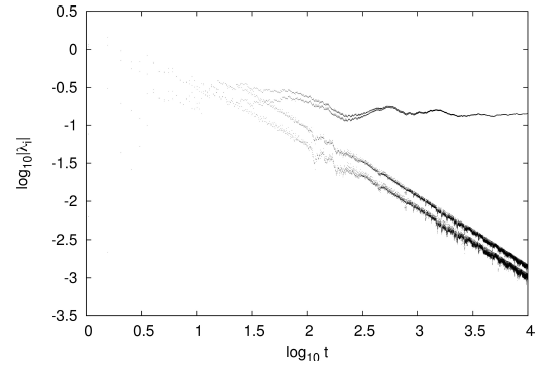
Fig. 1 LCEs of an orbit in the potential of equation (3) with parameters v ₀ = 1, q = 0.9, R _c = 0.14 and R _e = 3, started at the phase space point (x, y, x˙, y)˙= (0.1,0.5,0,1). From top to bottom, the sets of dots are generated by deviation vectors originally pointing along the directions ex,ey,ex˙ and ey˙, respectively. All the computations were performed with double precision. Since we are plotting the absolute value of the LCEs, if two of them were the opposite of the other two -as expected for a Hamiltonian system- only two sets of dots would be seen. 

4. THE SOLUTION

An important property of Hamiltonian dynamics is that Poincaré invariants are preserved along the flow (e.g. ^{Tabor 1989}). Let q and p stand for the coordinates and momenta of a canonical set, respectively; in addition, let C ₁ be any closed curve in the n-dimensional phase space encompassing a tube of orbits, and C ₂ any other closed curve enclosing the same set of trajectories. The first Poincaré invariant can be expressed as

We note that C ₂ could be the curve C ₁ evolved in time. Let us take, to fix ideas, n = 2 and Cartesian coordinates (q,p)=(x,y,x˙,y˙). If we choose for C ₁ the unit square in the plane (q1,p1)=x,x˙ at t ₀, it will enclose the area spanned by δ w _x (t ₀) and δ w _x˙ (t ₀), and the Poincaré first invariant will have only the term corresponding to x˙⋅dx. Furthermore, by virtue of Stokes’s theorem, the line integral will be equal to the enclosed area. If we choose the initial deviation vectors as before (unit vectors pointing along each Cartesian axis), this area will be equal to one, and by the invariance of the integral the area of the parallelogram spanned by δ w _x (t) and δ w _x˙ (t) for any t > t ₀ will remain unitary.

Now, the orthogonalization of the Gram-Schmidt algorithm allows us to compute the area of the parallelogram spanned by δwxt and δwx˙(t) as simply αx⋅αx˙, and since this area should be always equal to 1, we should have

for all t. The same will happen with the y coordinate. Looking at equation (1), we see that the deviation vectors started on the x and x˙ axes will give a pair of opposite LCEs, while those started on the y and y˙ axes will give the other pair.

But here we see the problem. On the one hand, as we have just seen, if for example δ w ₁ = δ w _x , then we must have δw4=δwx˙ in order to obtain the pair of opposite LCEs. But, on the other hand, this is not necessarily the order in which they are entered into the Gram-Schmidt routine. If these vectors are not the first and fourth, we are forcing the algorithm to find an opposite value of λ ₁ with a vector that is not the expected one, thus compelling the routine to give the correct modulus to a vector that was not the one that formed a unitary parallelogram with the first. This is numerically inefficient. Therefore, since the first and last deviation vectors inserted into the Gram-Schmidt routine should give the maximum LCE and its opposite sibling, they should be those originally pointing along a Cartesian coordinate and its corresponding velocity (in any order among them). The same occurs for the second and penultimate vectors, etc.

Figure 2 shows the LCEs of the same orbit as in Figure 1, but computed with the deviation vectors ordered originally in the directions (ex,ey,ey˙,ex˙). There are four sets of points plotted in the figure, generated by the evolution of those vectors. But the sets generated by ex and ex˙ are superimposed, so only one set is visible (the top one in the figure). In the same way, the two sets generated by ey and ey˙ are superimposed (the bottom set in the figure). Thus, we can see that the very same algorithm with the same orbit used before gives now exact opposite LCEs, as expected.

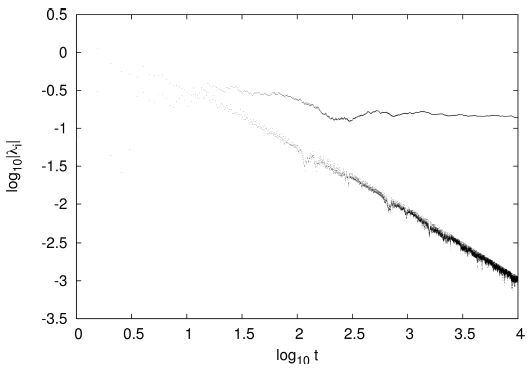
Fig. 2 LCEs of the same orbit of Figure 1, but starting with unitary deviation vectors δw1=ex,δw2=ey, δw3=ey˙ and δw4=ex˙. The top set of points were generated by ex and ex˙, though they are the same, so a unique set is seen. The same for the bottom set, which is a superposition of the sets generated by ey and ey˙. 

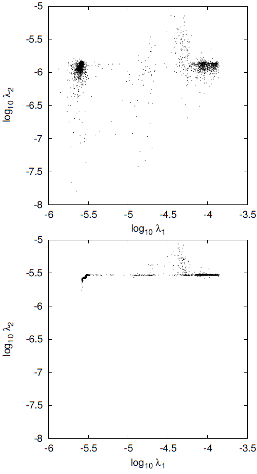
Besides, using the order of the initial vectors that we propose has the additional and more practically useful advantage that it yields better defined values of the computed LCEs. As an example, we computed the LCEs of orbits in the perturbed cubic force model used by ^{Muzzio (2017)} with −0.166843 < e ₁ < −0.166507, −0.324941 < e ₂ < −0.323994 and grid spacings ∆e ₁ = 2⁻¹⁷ and ∆e ₂ = 2⁻¹⁶ (see ^{Muzzio, 2017}, for details). The integrations were done for 5×10⁶ time units in all the cases. Figure 3 presents the resulting λ ₁ versus λ ₂ with the usual ordering (top panel), and the same with our ordering (bottom panel). Clearly, the dispersion of the λ ₂ values is smaller and their value better defined with our ordering of the initial vectors.

Fig. 3 Top: logarithmic plot of the largest (λ ₁) versus the second largest (λ ₂) LCEs for a perturbed cubic oscillator (see text for details) using the standard ordering of the deviation vectors. Bottom: the same but using the proposed ordering of the deviation vectors. 

5. CONCLUSION

The results obtained for the LCEs of a Hamiltonian autonomous system with the ^{Benettin et al. (1980)} method depend on the order used for the initial deviation vectors. To obtain the expected opposite pairs of LCEs, the deviation vectors should be ordered by pairs, the first, second, etc. ones having to be conjugate with the last, the penultimate, etc., respectively. The results obtained with such an ordering have the additional advantage of resulting in better defined values of the computed LCEs.