


 nueva página del texto (beta)
 Inglés (pdf)
 Artículo en XML
 Referencias del artículo
 Enviar artículo por email
 Citado por SciELO
  Similares en
SciELO
Similares en
SciELO 
 Permalink
1. Introduction
Simulating physical phenomena is a fundamental tool in engineering and the physical sciences, as it allows us to understand and predict the behavior of systems under different conditions. In many cases, the simulation of physical phenomena requires the use of large amounts of computational resources due to the quantity of data and mathematical operations involved. Therefore, it is important to consider the computational cost, especially if accurate results are desired in a reasonable amount of time. As a consequence, the selection of the most appropriate software tool that make the most of available resources is also an important desicion. There are various software tools available for this purpose, each with its own strengths and weaknesses. In this study, we compare the performance, efficiency, and resource usage of COMSOL Multiphysics and the MPh library of Python in the simulation of physical phenomena.
COMSOL Multiphysics is a widely used multidisciplinary simulation software that offers an extensive range of tools for the simulation and analysis of physical systems [1,2]. It is commonly used in engineering and materials science problems and has applications in a vast number of areas in physics, chemistry and engineering. One of the main advantages of COMSOL is its user-friendly graphical interface, which makes it easy to use for those with little programming experience.
On the other hand, Python is a general-purpose programming language that is widely used in data science and engineering. It is a very powerful and flexible language that offers a large number of libraries and modules for the simulation and analysis of physical systems [3]. In addition, Python has a large user community and extensive documentation available online. Nevertheless, Python requires programming skills and may be more difficult to use for those with little programming experience. A feature opposite to that of COMSOL is that Python and its libraries are open-source and free software, which means they can be used for free by anyone. Information and documentation about the Python programming language may be found at its website [4].
Due to the growing popularity of this programming language, the use of Python has been spread to many areas of application. Precisely, Python has a library to access the COMSOL API (Application Programming Interface). This library enables operations such as loading a model from file, reading and modifying parameters, solving the model and running the simulation, evaluating the results and exporting them. The library is named MPh. Information about this library and the way how to use its diverse functions is found in Ref. [5]. The relation between the MPh library of Python and COMSOL Multiphysics is depicted in Fig. 1. The physical model to solve is created in the COMSOL graphical user interface. The model and all its settings and parameters are saved in a *.mph file. This file may be manipulated either by COMSOL or Python. If we intend to solve the model using Python, the MPh library interacts with the COMSOL API to execute the numerical methods to yield the solution.
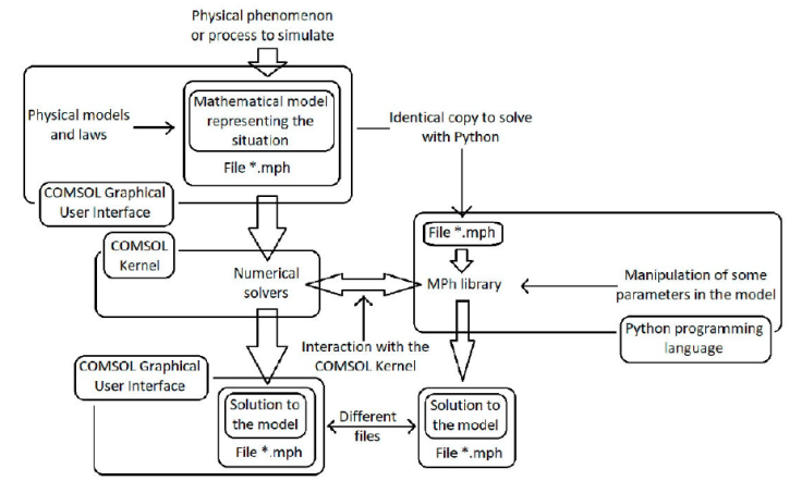
On the one hand, COMSOL comes with a modern graphical user interface to set up simulation models and visualize the results of the computations in a rich variety of 1D, 2D and 3D graphs. On the other hand, Python loads a file created by COMSOL containing all the parameters, information, and mathematical equations that describe the model, and also the type of analysis or solution we are looking for. Stationary, time-dependent, and parametric sweep studies are three such examples. All the manipulations to the model in Python, including the operations to load and solve it, are done through instructions typed in the Python interpreter. Obviously, this is an advantage of Python over COMSOL with regard to the demand of computer resources from the point of view of the user interface. We remark that the MPh library of Python does not replace the use of COMSOL Multiphysics, as this is just a bridge to the core that solves the mathematical equations. The creation and setting up of a model must be done in COMSOL, and additionally its powerful graphical user interface and features facilitates the visualization, manipulation and exporting of the data resulting from the simulation.
In this study we aim to determine which of these two software tools is more efficient for solving models of physical phenomena in terms of performance and computer resource usage. We focus on a specific physical phenomenon, the generation of magnetic field from a distribution of currents and ferromagnetic materials, to maintain the same conditions necessary for a correct comparison. Notwithstanding, it is very feasible that the results obtained can be extrapolated to the general solution of physical models. By comparing these two software tools, we hope to provide insights into the strengths and weaknesses of each one and help researchers and engineers to choose the most appropriate tool for their needs. The rest of the article describes the metrics used to compare the demands of computer resources when both software solve the same mathematical model, the characteristics of the computer equipment employed, the technique to scan the performance of the programs at solving, and the results obtained out of the comparison. Additionally, it is included a brief description of the physical phenomenon to simulate and its associated mathematical model to be solved.
2. Metrics for the comparison, its implementation, and the computer equipment
There are several software tools to monitor and record the performance and usage of the resources in a computer, and to scan the computer resources consumption by a specific process or program. Each one of these tools has its own features; features that allow to select, measure or record among some of the computer resources we want to monitor. In conducting this research, we decided to program our own process monitoring tools. These are two programs that conform to the measurement of the metrics defined below. The programs were coded in Python.
2.1. The metrics and its implementation in the monitoring-process program
Generally speaking, metrics are simply quantitative measures used for comparing, tracking, and understanding the performance of a specific process. The metrics considered in this work are CPU (Central Processing Unit) usage, RAM (Random Access Memory) usage, total execution time, and the size of the files with the solution data included. In addition, we consider the accuracy of the solutions provided by COMSOL and Python contrasted against each other, and with a known solution provided by the theory of electromagnetism. Before to define precisely each one of the metrics and how we implemented the measurement of them, we make a short digression about the library of Python named psutil (Python system and process utilities).
Psutil is a cross-platform library for retrieving information on running processes and system utilization (CPU, memory, disks, network, sensors) in Python. It is useful mainly for system monitoring, profiling, limiting process resources and the management of running processes. The documentation related to the characteristics and functionality of this library may be consulted in Ref. [6]. Several functions of this library were employed to measure the different metrics.
CPU (Central Processing Unit) usage. This refers to the amount of work that is being handled by the CPU, or how much of the computer processing resources are being used. This is usually measured as the amount of time a CPU spends processing the task of interest in a specified time length. We implement the measurement of the CPU usage with the function psutil.cpu_percent() which returns a float number representing the current system-wide CPU utilization as a percentage. An interesting fact about psutil.cpu_percent() is that the number returned by this function may be greater than 100. The reason is that the function sums up the CPU usage percentage of each individual core in a multiprocessor CPU. In order to obtain a number less than or equals to 100 (hence a true percentage), we have to divide by the number of logical processors of the computer equipment. In this article, we show the number returned by psutil.cpu_percent() directly.
Just as a remark, although the use of GPUs (Graphics Processing Units) was originally designed to accelerate the rendering of 3D graphics, over time they became more flexible and programmable, improving their capabilities this way. Now, GPUs are being used in a broad range of applications, like artificial intelligence, deep learning, and to accelerate additional workloads in high performance computing, besides graphics and video rendering [7]. However, in this article we only deal with CPU usage and not with GPU usage. This is due to the fact that COMSOL Multiphysics does not support the use of GPUs [8].
Memory usage. The term stands for the amount of memory that an application uses while running. In this case, the method memory info().rss of the class psutil.Process returns the non-swapped physical memory (RAM) a process has used in bytes. At this point, it is important to highlight that the most important factor in COMSOL Multiphysics to solve large models is to have enough physical memory (RAM), and that the RAM is correctly installed. If there is not enough RAM, then there will be significant slowdown, regardless of all other hardware choices [8]. For this reason, it is very relevant to monitor the RAM memory usage for COMSOL and Python.
Total execution time. It is the time interval that lasts the computation of the solution of a mathematical model. We measure this magnitude in seconds. In COMSOL, after the running of a simulation or computation has finished, the execution time, in seconds, is displayed. We took directly this value. With respect to Python, we used the function time.time() twice, once to record the beginning and the other to record the ending of the process. The function time.time() returns the time as a floating point number expressed in seconds since the epoch, in Coordinated Universal Time (UTC). The epoch is the point where the time starts; it is January 1, 1970, 00:00:00 (UTC) on all platforms.
Size of the saved files. This is the size of the files in bytes after solving the mathematical model and saving the solutions. File sizes are displayed by the operating system. At the beginning, a model is created in COMSOL and saved in a file without being solved. The file just contains the model, and the configuration needed to execute the numerical methods in a later step. Then, we make a copy from this original file to obtain two identical files with the same size on the file system. We solve one in COMSOL and the other one in Python. Both files are saved and their new sizes are compared. This metric allows to see how efficiently each software stores the final data.
Accuracy of the solutions. In order to validate the models and simulations, it is a common practice to contrast the result of the numerical solutions and calculated parameters against analytic known solutions and values also known from direct experimentation. All results computed by the MPh library are returned as NumPy arrays. NumPy is another library of Python employed for scientific computing. Information about NumPy can be found in its website [9]. We opened the data files to check and compare the contents of these files regarding the precision, and quantity of data saved in them. The MPh library of Python also allows the direct evaluation of a parameter if we know the name given to the parameter by COMSOL. In this work, we compared the magnetic force between two current-carrying wires calculated numerically by both software against the value known from the electromagnetic theory.
2.2. The computer equipment
The computer equipment employed in the present analysis is a Dell Inspiron 15 3501 laptop. The CPU inside the computer is a 11th Gen Intel(R) Core(TM) i5-1135G7 @ 2.40 GHz 2.42 GHz. This CPU contains 4 cores or independent CPUs and an 8 MB Intel Smart Cache [10]. It is possible to consider 8 logical CPUs in the equipment. “Logical CPUs” means the number of physical cores multiplied by the number of threads that can run on each core (this is known as Hyper Threading) [6,10].
Regarding the RAM, the laptop has two memory slots for inserting the cards. In one slot, there is an 8 GB memory card, and a 16 GB card in the other. In this way, the computer has a total of 24 GB RAM memory. The type of RAM cards is DDR4. The memory controller frequency is 6 MHz approximately.
The computer employed has the Microsoft Windows 11 Home Single Language operating system, the 10.0.22621 version. In addition, the COMSOL Multiphysics version used in this study was 5.6 version.
3. Methodology
Once established the metrics for the comparison, and the relevant characteristics of the computer used to run the programs, we explain the procedure followed to generate the information for the analysis. We investigated the demands of computer resources by COMSOL and Python through the execution of four different models saved in eight files. Initially, two identical files per model. The physical problem to solve and its associated mathematical model will be described in the Sec. 4. The first two files, containing the model 1, compute the magnetic field of a distribution of current due to a couple of solenoids and within the presence of ferromagnetic material. The second pair of files, containing the model 2, also include a magnetic sextupole defined by the ferromagnetic material and excited by additional current-carrying wires. These four files allow to monitor the demands of CPU and of RAM memory because the execution of the numerical solver takes a time of about 10 min and 2 h, for model 1 and model 2 respectively. As stated in the Sec. 2, the measurement of the CPU usage is defined employing a established time length for observation. The time interval between successive calls to the monitoring function of the CPU usage is 1 second. This is also the time interval between calls to the memory usage function.
The execution of the remaining four files lasts only a couple of seconds, being useless for the performance comparison. However, these files enable us to check the accuracy of the solutions. The first two files, corresponding to model 3, compute the magnetic field of a single solenoid. This model is useful in order to compare the accuracy of the solutions provided by both programs. The last two files model two parallel current-carrying wires separated by a given distance. In this model, apart from the field computation, the magnetic force computation between the wires is performed. The force between the wires is known from the theory of electromagnetism, hence we have a value to compare with the numerical solutions.
4. Physical problem and mathematical model
In this section, we briefly describe the mathematical model to be solved using numerical methods. The four models employed in this work all deal with the calculation of the magnetic field B due to a current distribution and within the presence of ferromagnetic materials. Model 4 also provides the value of the total magnetic force between two conductors one meter apart. Strictly speaking, the magnetic field is represented by the variable H, and B is known as the magnetic flux density. H and B are related by the so-called constitutive relations. Through these constitutive relations, the macroscopic electric and magnetic properties of the medium are described. The equation that allows to compute the magnetic field as a consequence of the presence of distributions of electric current, magnetic materials and electric fields is Ampère’s law:
where J is the electric current density, and D is the electric displacement field. Just as H and B are related by a constitutive relation, in the same way D and E, the electric field, are related by their respective constitutive relation that determine the electrical properties of the medium. Usually, in the presence of materials with isotropic linear electric and magnetic properties, the constitutive relations are
𝜖0, 𝜖 r and 𝜖 are three scalar quantities, the electric permittivity of vacuum, the relative permittivity, and the electric permittivity of the medium, respectively. Similarly, μ 0, μ r and μ are scalars and are known as magnetic permeability of vacuum, relative permeability, and magnetic permeability of the medium, respectively. Most of the region in which the magnetic field is calculated contains linear and isotropic magnetic materials; therefore, they are described by giving the value of μ. The ferromagnetic material used in the simulation has a nonlinear behaviour, and is modeled according to
The form of the function f(||H||) must be entered into the model. Finally, the current density J is given by
with σ the electrical conductivity of the medium, and J e an externally generated current density.
The specific problem we dealt with in the COMSOL models comes from magnetostatics. In the magnetostatic case, and without electric fields present, we have ∂ D /∂t = 0, E = 0. Thus, Ampère’s law Eq. (1) and the current density Eq. (4) take the form
Equation (5) represents the physical situation to be analyzed. Most of the solution methods, and this is the case in COMSOL Multiphysics, solve Eq. (5) putting it in terms of the magnetic vector potential A. This is done through the change of variables: H → B → A. The change of variable H → B is done via the constitutive relations like Eqs. (2) and (3). The definition of the vector potential provides the missing relation
Using the definition of vector potential Eq. (6) and the constitutive relationship Eq. (2), we rewrite Ampère’s law as
Equation (7) is the mathematical model that COMSOL solves using numerical methods. Once the solution for A is obtained, it is easy to get the solution of B, it is just a matter to use Eq. (6).
The method to obtain the force between two current-carrying conductors implies no more heavy calculations. The force is calculated via
f is the volume force density, J is given by the user when the model is configured, and B is computed via Eqs. (7) and (6), which is the time-consuming and hard part of the computations. In order to obtain the total force a wire experiences by the other wire, it is necessary to perform a numerical volume integral in the region defined as part of the wire.
A more detailed explanation of the physical meaning of the magnitudes appearing in Eqs. (1)-(8), and of the Eqs. (1) - (8) themselves and their consequences, may be found in texts about electromagnetism. Two classical books are Introduction to electrodynamics by David J. Griffiths [11] and Classical electrodynamics by John D. Jackson [12]. The first book has an undergraduate level, while the second one is intended for graduate studies. Table I summarizes the electromagnetic quantities appearing in this section with their respective SI units.
Table I Electromagnetic magnitudes involved in the mathematical model to be solved for finding the values of B in a region of space and their SI units.
| Variable | Magnitude | SI unit |
|---|---|---|
| B | Magnetic flux density | Tesla (T) |
| H | Magnetic field strength | Amp ere/meter` (A/m) |
| E | Electric field strength | Volt/meter = |
| Newton/Coulomb | ||
| (V/m = N/C) | ||
| D | Electric displacement | C/m2 |
| J | Current density | A/m2 |
| A | Magnetic vector potential | Weber/meter (W/m) |
| t | Time | Second (s) |
| μ, (μ 0) | Magnetic permeability | Henry/meter (H/m) |
| (of vacuum) | 4π × 10-7 H/m | |
| 𝜖, (𝜖 0) | Electric permittivity | Farad/meter (F/m) |
| (of vacuum) | 8.85 ×10⁻¹² F/m | |
| μr, 𝜖 r | Relative permeability | Dimensionless |
| and permittivity | ||
| σ | Electrical conductivity | Siemens/meter (S/m) |
| f | Volume force density | N/m3 |
Regarding the form of how the COMSOL kernel is programmed to solve the systems of differential equations resulting from the physical models, and the numerical solvers the kernel uses for this purpose, there is information available on the COMSOL Multiphysics website [1]. Some good starting points are [13-16]. The principal reference that describes all the aspects of COMSOL Multiphysics is the COMSOL Multiphysics reference manual. The manual is also available on the COMSOL website.
5. Results
The data recorded from the execution of COMSOL and Python when solving the mathematical models described in Sec. 3 are shown in the next graphs. Figures 2 and 3 show the performance of the CPU and memory demand at solving the model 1. Figure 2 shows that the CPU demand is lower in Python than in COMSOL most of the time. The mean CPU usage throughout the execution of the programs is 324.0% by COMSOL and 303.6% by Python. It is also possible to appreciate that the distribution of the data obtained from each software, displayed in the graph of Fig. 2, is quite similar. The standard deviation confirms this assumption: σ com = 46.9 and σ mph = 47.5. σ com, σ mph stand for the standard deviation of the data obtained by running COMSOL and Python, respectively. We continue with the analysis of the next metric, the RAM memory demand. Likewise to the CPU usage, Python employs less RAM memory than COMSOL. Despite the lower memory consumption by Python, the RAM presents the same usage patterns by COMSOL and Python, confirming effectively that the same algorithms are executed in both programs. Note that the horizontal axis of the graphs in Figs. 2 and 3 do not represent the execution time of the programs. What is represented by this axis is the number of times a system call has been made to read both CPU and memory usage. We call this operation an iteration. The algorithm of the monitoring program includes a routine to wait for one second before performing the next iteration. Despite the above, we can not expect the time interval between two iterations to last precisely 1 s. Between two iterations the program performs various tasks with the data obtained from the system calls, and even worse, the monitoring program creates two threads that run at the same time and only one of them makes the system calls. It depends on the operating system how long each thread is executed by the CPUs before switching to the other or to another process, and therefore, the execution times between iterations is variable. Anyway, the iteration number gives an estimation of the execution time of the program. In order to solve the model 1, COMSOL took a time of 698 s. The time spent by Python to fulfill the same task was 714 s. The last metric we consider in this work is the file size of the model generated after solving it. The file generated by COMSOL has a size of 99,438,907 bytes ≈ 94.8 MB, the one generated by Python, 53,002,007 bytes ≈ 50.5 MB. The file generated by Python has almost the half of the size of the file obtained with COMSOL. Table II summarizes the values of the metrics obtained from monitoring the four models.
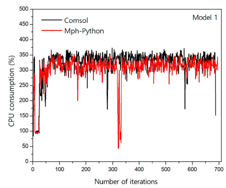
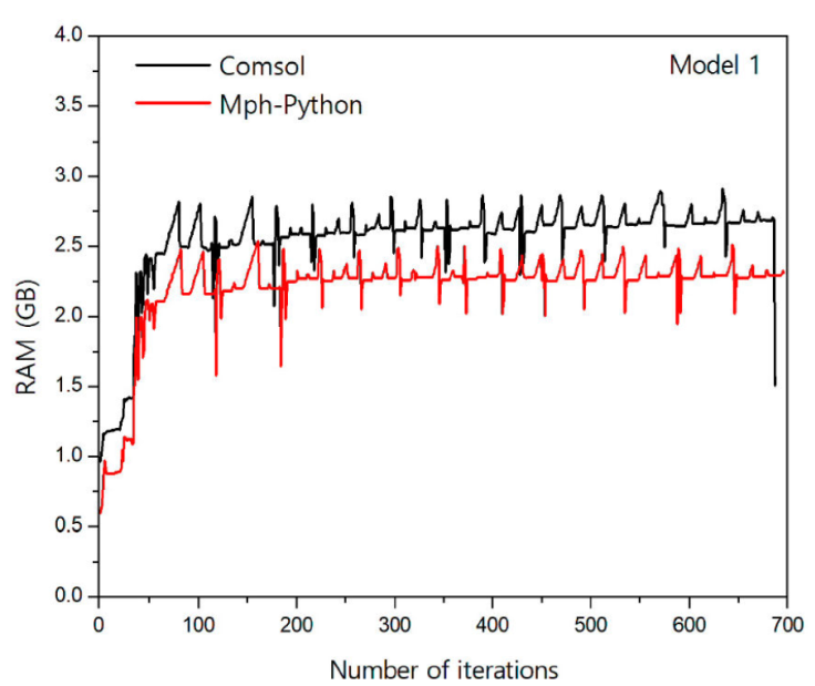
Table II Summary of the metrics of the 4 models. The upper data in each entry is from the model solved by COMSOL. The initial file size is the same for both.
| Model 1 | Model 2 | Model 3 | Model 4 | |
|---|---|---|---|---|
| Minimum | 83.6% | 60.6% | 28.1% | 114.9% |
| CPU usage | 43.3% | 22.2% | 165.2% | 131.9% |
| Maximum | 372.8% | 423.9% | 432.6% | 498.6% |
| CPU usage | 366.0% | 372.8% | 346.7% | 363.8% |
| Mean | 324.0% | 320.3% | 228.4% | 275.8% |
| CPU usage | 303.6% | 298.7% | 250.5% | 240.4% |
| Minimum | 0.96 GB | 1.04 GB | 843.04 MB | 813.15 MB |
| RAM usage | 0.60 GB | 0.78 GB | 683.37 MB | 750.86 MB |
| Maximum | 2.91 GB | 12.17 GB | 1020.76 MB | 1014.32 MB |
| RAM usage | 2.54 GB | 12.41 GB | 868.88 MB | 1084.95 MB |
| Mean | 2.54 GB | 9.09 GB | 932.33 MB | 926.83 MB |
| RAM usage | 2.20 GB | 9.08 GB | 795.12 MB | 961.33 MB |
| Execution | 698 s | 6344 s | 3 s | 2 s |
| time | 714 s | 6105 s | 6 s | 5 s |
| Initial file | 13.86 MB | 142.95 GB | 0.90 MB | 0.19 MB |
| size | ||||
| Final file | 94.83 MB | 418.95 MB | 4.38 MB | 1.45 MB |
| size | 50.55 MB | 185.69 MB | 1.58 MB | 0.18 MB |
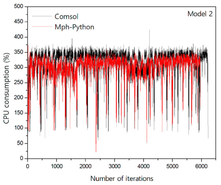
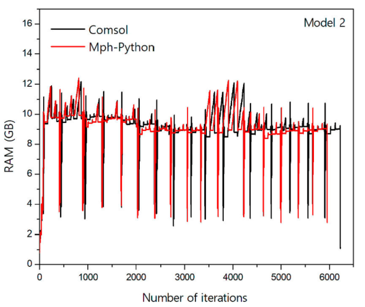
Now, we proceed to carry out a similar analysis to that of model 1 with model 2. Figures 4 and 5 show the CPU and memory performance when solving the model 2. Figure 4 shows again that Python demands less CPU usage. On average, Python uses 298.7% of the CPU and COMSOL uses 320.3%. Dispersions of the data given by their respective standard deviations are σ com = 43.6 and σ mph = 41.5. A dispersion of data quite similar in both cases. Figure 5 shows a consumption of RAM very similar between the two programs. First, as in the previous case, RAM usage behaviour patterns are almost identical, confirming once again the execution of the same numerical methods. Second, in this model the amount of RAM used by Python and COMSOL is almost the same. Even Python had a slightly higher maximum memory consumption than COMSOL. Despite the above, most of the time Python consumed less RAM. In summary, the observations made to the execution of model 2 reinforce the thesis that Python makes a better use of CPU and RAM. We now continue with the next metric, the execution time. In this case, the execution of COMSOL solving the model is longer than that of Python. COMSOL employed 6344 s to complete the task, whereas Python used 6105 s. Finally, the sizes of the resultant files are 439,303,098 bytes ≈ 419.0 MB the COMSOL file and 194,712,992 bytes ≈ 185.7 MB the Python file. The Python file has approximately the half of the size than the COMSOL file. The values of the metrics for the model 2 appear in Table II.
In Sec. 3, it was explained that models 3 and 4 are not appropriate for the analysis of CPU and RAM usage due to the very short execution time of the programs when solving the models. However, the metrics of these models appear on Table II. One of the two metrics considered for the analysis in these two cases was the file sizes. In both models, models 3 and 4, COMSOL final file sizes are much larger than the equivalent Pyhton file sizes. In model 4, even the Python final size is smaller than the original file size. Therefore, another conclusion we can make is that Python has a greater performance in the storage of data.
In COMSOL Multiphysics, the solution dataset may be exported into a text file. Similarly, Python handles the solution dataset as a NumPy array, and this array may also be stored in a text file. In a later step, text files can be opened and compared. The results of the inspection of the files are described next. The solution dataset of model 3 consists in 15,600 nodes in both files. The numerical data stored in the files are exactly the same. Nevertheless, the inspection result of the files corresponding to model 4 was unexpected. In this case, the number of nodes stored in the COMSOL dataset is 452, in contrast to the 6323 nodes in the Python dataset. It turns out that the COMSOL dataset is a subset of the Python dataset. The numerical precision employed in both datasets is the same. This results reinforce the picture illustrated in Fig. 1, the MPh library of Python employs the kernel of COMSOL to solve the models. In order to appreciate the accuracy of the solutions provided by the software, in the model 4, the force exerted by one cable on the other according to the electromagnetic theory is 2.0 × 10⁻⁷ N/m. The value provided by both software is 1.9966301423761032 ×10⁻⁷ N/m.
6. Conclusions
Table II shows that Python is more efficient in each and every one of the metrics employed for the comparison. The CPU mean usage difference between COMSOL and Python was 40%. Figures 2 and 4 and the consideration of the standard deviation of CPU usage data highlight a similar pattern of CPU consumption. Analogously to the CPU case, the use of RAM memory follows the same behaviour pattern as shown in Figs. 3 and 5. The overall demand of RAM by Python was less than by COMSOL, though in model 2 the difference is very small.
The size of the files containing the solved models was smaller in Python in all the cases. In three of the four models, the Python files were about the half of large than COMSOL files. Regarding the execution time of the programs, the behaviour of the programs is not clear. Sometimes the execution time is smaller in COMSOL, some other times in Python. Either way, the time length is similar when measuring in seconds. Finally, the precision of the solutions given by both programs is exactly the same. In the case of model 3, the amount of data was also the same. At the other hand, the amount of data exported by COMSOL for model 4 was only the 7.15% of that of Python.
In conclusion, we remark that when using the MPh library of Python we can not omit the use of COMSOL. In the first place, the creation of the models with their adequate adjustments to solve them are done in COMSOL. Secondly, Python employs the COMSOL kernel to solve the models numerically. Despite the above reasons, Python is more efficient at solving the models. As a result, we can also conclude that the most efficient way to perform the simulations created with COMSOL Multiphysics is to solve them in Python. Finally, with the solutions at hand, we can manipulate the data in whichever tool we prefer, or according to our needs.

