1. Introduction

The interaction between light and the earth’s atmosphere offers the human eye a vast number of beautiful images that reveal a wide variety of optical phenomena. Well-known examples are rainbows, halos, coronas, or the twinkling of stars [¹]. All of them are manifestations of the pass of electromagnetic radiation through the matter that compose the Earth’s gaseous envelope in very specific meteorological situations, different from each other, and particular positions of the observer. Nevertheless, they have in common that they are related, to a greater or lesser extent, to the refraction of light, an unavoidable issue in disciplines such as astronomy, geophysics, and meteorology when dealing with the propagation of radiation in the atmosphere. For example, atmospheric refraction is of primary importance in studies related to imaging of astronomical sources [¹⁶], geolocation [¹⁵] or remote sensing [⁹].

Among the most known optical phenomena are the inferior mirages, which are often observed on sunny days on highways and deserts. As a consequence of a great heating of the ground surface by solar radiation, there is a strong temperature gradient in the air layers closest to the ground that deviates the rays’ paths through them. A possible way for studying inferior mirages is the calculation of the trajectories followed by light rays in refractive media. To do this it can be used, for example, methods that involve differential equations derived from the variational principle, in analogy with Newtonian mechanics, considering a variable refractive index [³,⁴]. Other more modern computational techniques based on ray tracing, and which simulate the behavior of the atmosphere, can also be found in the literature [²,⁶,¹⁴]. Some authors have also developed models that are able to determine vertical temperature variations near the ground from direct observation of a mirage [⁵, ⁸, ¹¹]. In a previous work [¹⁰] we have developed a methodology that makes it possible to obtain the path of the light rays during the mirage by using a simple analytical expression, derived from Fermat’s principle, that takes into account the behavior of the air in the microlayer (small portion of the atmosphere a few centimeters thick that is in contact with the Earth’s surface). This type of treatment includes, as a key element, the determination of the vertical profile of the refractive index from atmospheric variables (pressure and temperature) and the wavelength of light. For modeling the atmospheric influence on the refractive index, physical considerations of heat transport in the microlayer are made.

Using our technique, we have previously analyzed the possible limits of observation of the phenomenon, expressed in terms of minimum/maximum distances. In the present work, we study what observers perceives when they are located at different positions in a vertical plane perpendicular to the surface. Through an analytical treatment, Khular et al. [⁷] already showed that, depending on the position of the observer, she or he could receive a direct ray from the point object, a ray that has suffered atmospheric refraction (and which forms the inverted image of the object), both rays simultaneously, or neither. Furthermore, these authors showed that the locations of the regions where these different situations can occur varies greatly as the vertical profile of the refractive index changes (as a consequence of a variation of the temperature profile). However, the treatment they realized is rather descriptive and limits are not presented for the mentioned observation regions. The method we have developed allows to analytically describe the path of the outgoing rays from the object and to locate the observers for these rays in terms of distances to the object and heights from the ground. Thus, it is possible to propose limit situations that allow to distinguish positions for which direct and/or refracted rays may or may not be received. Through the application of our technique, we obtain analytical expressions that delimit the different observation regions of the phenomenon. Complementarily, since the model explicitly depends on meteorological conditions, we analyze how these regions vary for different atmospheric situations.

We organize this work as follows: in Sec. 2 we make a brief description of the calculation technique, presenting, first, the atmospheric modeling and, then, the analytical expressions that describe the ray paths; in Sec. 3, by considering all the refracted rays that emerge from a point object, we analyze how the position of the closest approach to the ground varies for them; in Sec. 4 we present the analytical expressions that describe the limits of the observation regions of the phenomenon and then apply them to analyze how they vary for different atmospheric situations; finally, Sec. 5 presents a brief summary of the results obtained and our conclusions.

2. Methodology

For the analysis of the inferior mirage, we consider the trajectory of the rays that emerge from a point object and travel downwards towards the ground. These rays are strongly deflected by atmospheric refraction when they are very close to the ground, what causes them to ascend and, eventually, reach the observer. The calculation of the ray path consists of two stages: the modeling of the atmosphere in the microlayer (where a significant temperature gradient takes place) at the time of the mirage, and the ray tracing itself. In this Section, we briefly describe these two instances; a more exhaustive description of this technique can be found in the work of Paola et al. [¹⁰].

2.1. Microlayer model

The atmospheric state near the ground depends on the heat transport mechanisms playing in the first layer of air. In our model, we consider that the total heat flux Q (W/m²) is the sum of the fluxes transported by molecular and turbulent processes, assuming the latter as a fraction of the former. Given the strong relationship between conduction and air temperature (T), the thermal conductivity of air is expressed as a function of the latter. After an iterative process, values of T (^◦C) are obtained in the first centimeters of atmosphere, which have a marked exponential variation with height, between the values T ₀ (surface) and T _f (field). From the values of T obtained, the vertical variation of the refractive index (n) is simulated using the following expression:

n-1=0.05792105238.0185-λ-2+0.0016791757.362-λ-2×(273+15)(273+T)P76 (1)

where P (cmHg) is the atmospheric pressure and λ (µm) is the wavelength of the light. It should be noted that all calculations in Paola et al. [¹⁰] were carried out assuming P = 76 cmHg and λ = 0.5 µm, being the latter a value close to the wavelength of the maximum of energy emission of the Sun and the maximum sensitivity of the human eye to light. In virtue of the strong relationship with T, the vertical variation of n is also exponential, and has the following expression:

n(y)=nf1-αexp⁡-yβ (2)

where y (cm) is the vertical coordinate (y = 0 on the surface), n _f is the refractive index in the field, and α (dimensionless) and β (cm) are positive constants. The parameter α is related to the variation amplitude of the refractive index, and it is expressed as follows:

α=1-n0nf (3)

where n ₀ is the refractive index at the surface. On the other hand, the parameter β indicates the rate of n growth with height, which, as showed in Paola et al. [¹⁰], is roughly equal to the rate of T decrease with height near the surface. Considering Eqs. (2) and (3), it is simple to prove the following expression:

β=y1ln(nf-n1)(nf-n0), (4)

where n ₁ is the value of the refractive index at y ₁ (cm), intermediate height between the surface and the field.

Since n variations are associated with meteorological variables, we can implicitly express the effect of the atmosphere on the phenomenon by means of constants α and β. However, we are interested on expressing both parameters in terms of measurable atmospheric variables. As different authors have shown [⁵, ⁸, ¹¹], it can be very useful to establish direct relationships between the characteristics of the phenomenon and the weather conditions. Using Eqs. (1)-(4) it is possible to show that parameters α and β can be obtained from temperature values. Rewriting Eq. (1) we obtain:

n=1+AT, (5)

where the temperature is now expressed in K, and the parameter A (K) becomes:

A=3.78940.05792105238.0185-λ-2+0.0016791757.362-λ-2P. (6)

If we adopt, as in Paola et al. [¹⁰], P = 76 cmHg and λ = 0.5 µm, A = 0.0786251686 K.

Using Eq. (5) for points on the surface, the field, and the intermediate height y ₁, where the temperature is T ₁, Eqs. (3) and (4) are rewritten as follows:

α=A(T0-Tf)T0(Tf+A)β=-y1lnT0(T1-Tf)T1(T0-Tf) (7)

Hence, to calculate the parameters that model the refrac tive index, it is only required the value of the temperature at three points. In this case, the amplitude of variation of n depends on the T ₀ and T _f values, while its growth rate is also determined by T ₁. Due to the rapid decrease of T with height [¹²-¹⁴], we assume that y ₁ = 1 cm. In order to illustrate the behavior of α and β we use Eqs. (7) to calculate both parameters, considering A = 0.0786251686 K and different temperature combinations. Figure 1 shows the values of α and β obtained as a function of T ₀ for different values of T _f (panels a and c), and as a function of T _f for different values of T ₀ (panels b and d), considering also different rates of variation of temperature with height (T ₁/T ₀ = 0.65 and T ₁/T ₀ = 0.85 in panels c and d). As expected, the obtained curves show that, for a given T ₀, α and β increase as T _f decreases (i.e., as the amplitude of temperature variation increases). For a given T _f , while α grows approximately linearly with T ₀, β grows fast for values of T ₀ close to T _f , and slower for larger differences between both temperatures. On the other hand, for a given pair of T ₀ and T _f values, β increases as T ₁ increases (i.e., as the temperature decreases with height more slowly). However, the values of β cannot be very large since, as mentioned before, on occasions of inferior mirages, the temperature drops very fast, and the field value is generally reached very close to the ground. Assuming 40^◦C ≤ T ₀ ≤ 70^◦C and 20^◦C ≤ T _f ≤ 45^◦C as reasonable values (i.e., not extreme in nature), as experimental and measured data suggest, through numerical simulations, we have approximately limited the variation of the parameters to the intervals 1.1 × 10⁻⁵ ≤ α ≤ 4 × 10⁻⁵ and 0.3 cm ≤ β ≤ 0.8 cm [¹⁰]. For a better visualization of the most expected values of α and β, in Fig. 1 are outlined the regions contained by those limits, making evident that not all combinations of parameter values are possible. It is worth mentioning that we also analyzed the influence of atmospheric pressure on the parameter α which, according to Eqs. (7), is the only one that has a direct relationship with P.

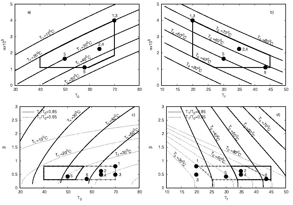
FIGURE 1 Parameters α and β as a function of the temperatures T ₀ and T _f . In panels c and d the curves are presented for two different T ₁ /T ₀ ratios (lines are plotted every 10 ^◦C). The closed curves at the bottom of each graph delimit reasonable values of α and β corresponding to most probable (i.e., not extreme) atmospheric situations, in terms of temperatures T ₀ and T _f (see text), and for both ratios of T ₁ /T ₀ in panels c and d. The numbered points represent different atmospheric situations that are considered in Fig. 7. 

On the one hand, the vertical variation of pressure is negligible in the microlayer [⁷], so it can be assumed constant. On the other hand, we observe that for the expected variation range of pressure on the earth’s surface (approximately 50 hPa; i.e., 3.75 cmHg) α presents a variation of less than 5%, so we can assume that pressure does not play a relevant role in the inferior mirages.

2.2. Ray tracing

The next step consists of calculating the light rays’ path from the refraction index profile obtained. This calculation is made using a simple analytical expression that is obtained by stating that, according to Fermat’s principle, the light travels an optical path that minimizes the time. To derive this expression, we consider as a reference frame a Cartesian system xy so that the x-axis (horizontal) has its origin (x = 0) at the place where the ray reaches its minimum height (y ₀). We call this point of coordinates (0,y ₀), where the ray begins to ascend, “V point”. Operating properly, it can be shown that the ray path is defined by the pairs (x,y) that arise from the following expression [¹⁰]

xy, y0=2βγln⁡1+1-exp⁡-y-y0β+γ(y-y0), (8)

where

γ=1-αexp⁡-y0β2αexp-y02β (9)

Since the second term of the numerator in Eq. (9) is much smaller than 1, Eq. (8) can be written as:

xy, y0=2βexp⁡(y02β)2α⁡ln⁡1+1-exp⁡-y-y0β+exp⁡(y02β)2α(y-y0) (10)

We only consider in our model a one-dimensional variation of the atmospheric variables, so that the ray path presents a symmetry with respect to the y-axis. Therefore, for negative values of x the descending part of the ray (i.e., from the point object to the V point) is represented, while for positive values the ascending part of it (i.e., from the V point to the observer eyes) is represented. For a better description of the ray path, we call d and h the horizontal distance from the point object and its height, respectively (see Fig. 2). Under this configuration, by replacing y by h in Eq. (10), we obtain the distance between the point object and the V point of height y ₀:

d(y,y0) = 2βexp⁡(y02β)2αln⁡1+1-exp⁡-h-y0β+exp⁡(y02β)2α(h-y0) (11)

and thus, the distance to the point of height y for the considered ray results:

d(y,y0)=dV(y0)+x(y,y0). (12)

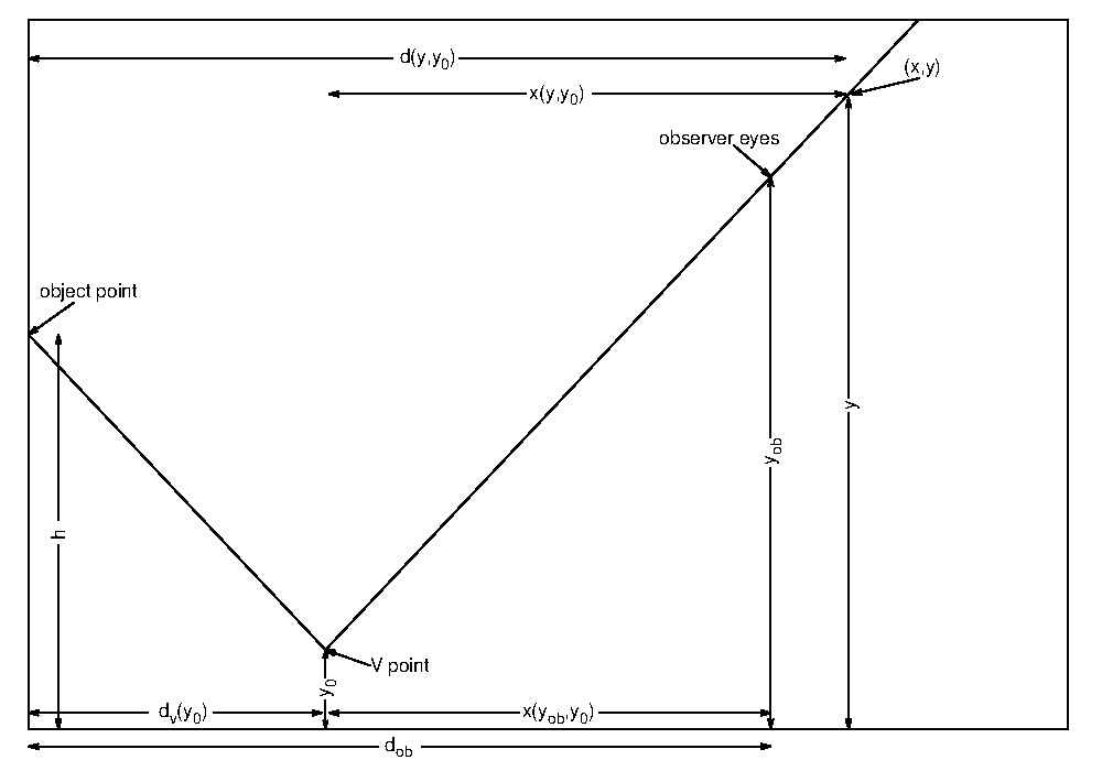
FIGURE 2 Path of the ray that, emerging from the point object, passes through the V point at height y ₀, and reaches the observer eyes at height y _ob . 

In particular, if we call y _ob the height of the observer eyes who receives the ray (or the device used to register the mirage), the distance obtained with Eq. (12) is the objectobserver distance (d _ob ).

3. Analysis of V point position for rays emerging from a point object

Let us consider the ray that, emerging from a point object located at a height h, passes through the V point characterized by y ₀. For this ray, an observer located at a smaller distance than d _V (with her or his eyes at the appropriate height) will only be able to see its descending part, and thus there is no possibility that this ray will contribute to the visualization of a mirage for this observer. Therefore, knowing the spatial distribution of the V points can be very useful to define regions where observers may be located to visualize the object and/or its image.

If we consider different rays emerging from the point object, we find that, as the angle that the rays form with the normal to the ground increases, the V points of these rays are characterized by progressively larger values of y ₀ and greater distances d _V [¹⁰]. However, this behavior does not extend infinitely since, according to Eq. (11), if y ₀ reaches the value of h, the distance d _V becomes zero. Therefore, there must be a maximum distance, d _Vmax hereafter, from which the V points (corresponding to y ₀ values increasingly closer to h) get closer to the point object (until reaching it). This can be verified in Fig. 3, that shows the curves joining the positions of the V points of different rays that emerge from a point object, being displayed a curve for each point object at a different height (h between 3 and 6 cm). For this example, we considered α = 1.10865 ×10⁻⁵ and β = 0.33 cm, which correspond to a temperature profile characterized by T ₀ = 58 ^◦C, T ₁ = 44.2 ^◦C (T ₁ /T ₀ = 0.76) and T _f = 43.5 ^◦C (this profile can be obtained assuming that the heat fluxes transported by turbulent and molecular processes are equal at a height of 1 mm, being the total heat flux Q = 260 W/m²).

FIGURE 3 V point positions for rays emerging from point objects located at different heights h. 

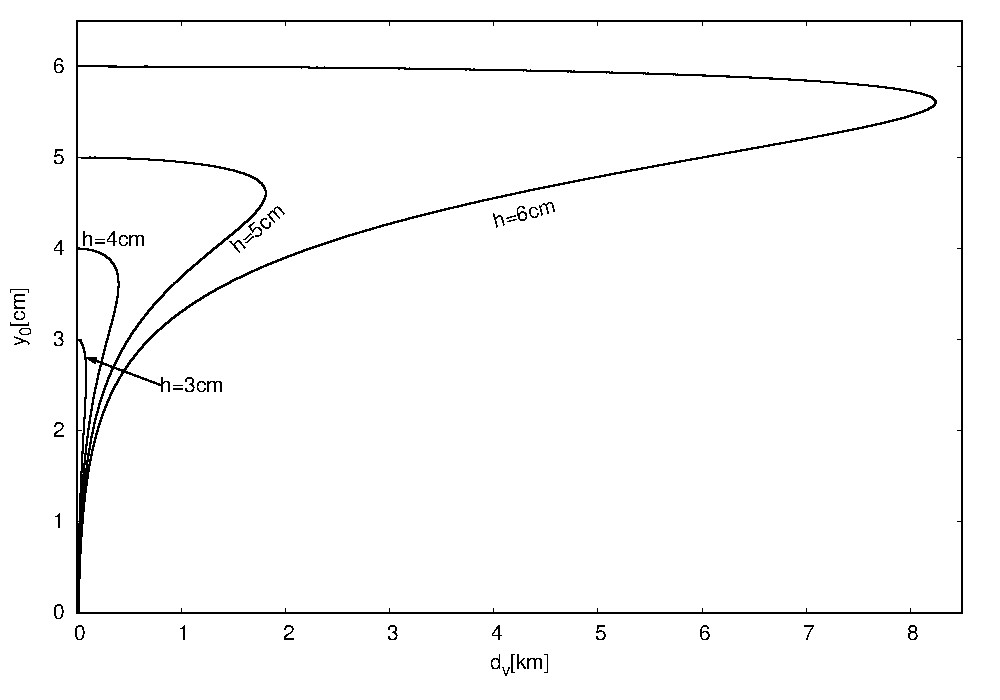
From Fig. 3 it is apparent that the maximum value of d _V grows very rapidly with small increases in the height of the point object. The value of d _Vmax can be analytically obtained by calculating the derivative of Eq. (11) with respect to y ₀ and setting it equal to 0. Calling m=1-exp⁡(-(h-y0)/β) and considering that exp(−y ₀ /β) «1, the following equation is obtained:

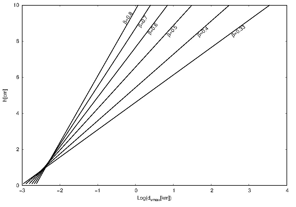
which has a unique solution for m = 0.8335. Since β is a positive constant, the term h − y ₀ for this solution takes a single positive value (for example, for β = 0.33 cm, h−y ₀ ≈ 0.39 cm), from which we can obtain d _V max using Eq. (11). Following this procedure, we calculate d _V max for different h and β values, being the results presented in Fig. 4. In addition to verifying the pronounced growth of d _V max with h (note the logarithmic scale of the abscissas-axis in the figure), it can be observed that this effect increases as β decreases. For h greater than a few centimeters, the distances obtained are extremely large and cannot be considered within the range of our analysis (because of the limitation imposed by the effect of the sphericity of the Earth, inter alia). Therefore, we start considering small values of h in analyzing the limits of the regions, in a plane perpendicular to the ground, in which an observer should be located to visualize the point object and/or the image.

FIGURE 4 Maximum distance of V points of rays emerging from point objects at different heights h, for different β values. 

4. Object and/or images visualization regions

In this section we analyze the configuration of regions in a vertical plane where an observer could see only images, only object, both or neither. To illustrate our analysis, we use Eqs. (10)-(12), considering α = 1.10865 × 10⁻⁵ and β = 0.33 cm, to calculate the paths of the rays that emerge from two point objects located at h = 5 cm and h = 7 cm. The ray paths obtained are presented in Fig. 5. For a better visualization of the results, we identify with dotted lines the segment from the point object to the V point, and with thin solid lines from the V point onwards. In the figure, we also indicate with thick solid lines the limits of the regions described below, which coincide with those identified in [⁷].

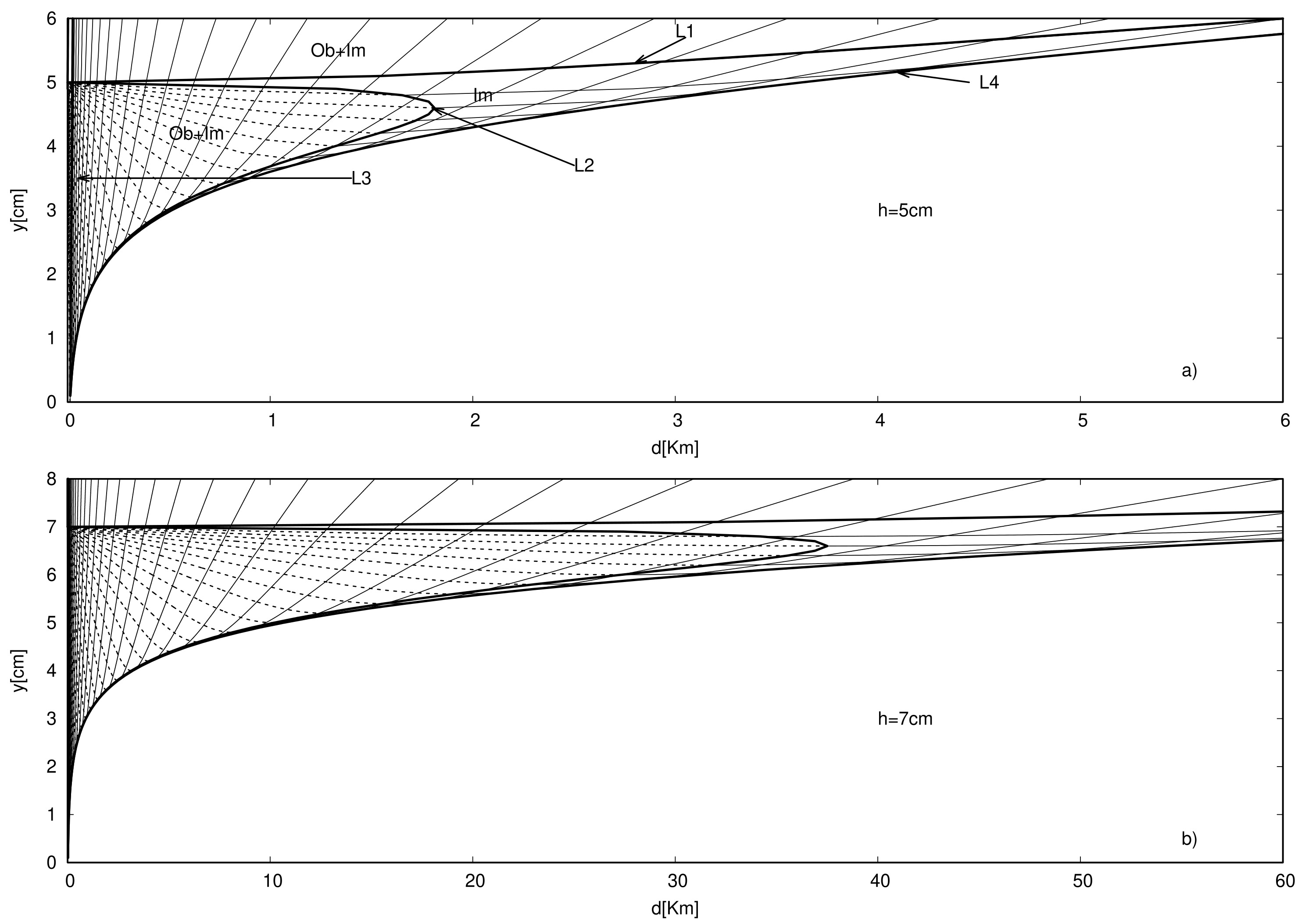
FIGURE 5 Paths of emerging rays from point objects located at h = 5 cm (panel a) and h = 7 cm (panel b). For description of curves L1, L2, L3 y L4 see text. 

The curve L1 corresponds to the first ray that, after emerging from the point object, does not present a descending part (i.e., the V point is where the point object is). Therefore, it represents the upper limit of a region where observers only see an image (above it, observers receive both, direct and refracted rays). The analytical expression for L1 is obtained by setting d _V = 0 which, as mentioned in the previous section, is given for y ₀ = h:

The curve L2 is the union of the V points of the computed rays (i.e., the one analyzed in the previous section). Any observer located at the same height, but at a greater distance than L2, do not receive any direct ray from the point object. Therefore, like curve L1, it represents a limit for the location of observers who can see only images. The analytical expression of L2 is obtained by calculating d _V for y ₀ = y _ob:

The curve L3 is built considering the first ray that, emerging from the point object, is not absorbed by the ground (i.e., the ray that barely touches the ground before starting its ascending part). Therefore, this curve represents the minimum distance at which an observer can see an image (for smaller distances, the observer only see the object). The analytical expression for L3 is obtained by setting y ₀ = 0:

In Eq. (16) the first term is much smaller than the second one for any values of h and yob, so that we can assume that the curve L3 is represented very accurately by the second term of that equation. This simplification was also obtained in Ref. [¹⁰] approximating the ray trajectories by their asymptote lines. It is also worth mentioning that, since the V points of the rays with y ₀ close to h are located progressively near the point object, the curve L3 departs from the nearly linear path in the vicinity of h. Close to h, L3 shows a wedge-shaped zone that gets between the curves L1 and L2 for smaller distances than those given by Eq. (16), where only the image of the point object can be observed. This zone is so small that it would be seen as a horizontal line at y = h in Fig. 5, from d = 0 to L3, and it is, thus, discarded from any analysis.

The curve L4 is built as the lower envelope of the ray paths, and thus, it represents the lower limit for the location of observers who can see an image. Below this curve there is an invisibility zone where it cannot be observed neither object nor its image. We propose to represent this curve, numerically obtained, by the following analytical expression:

where the parameters a, b and c are functions of h, α and β. From several numerical tests, considering h values between 1 and 300 cm and different α and β values, we obtain the expressions:

that allow fitting, with Eq. (17), the analyzed curves with error less than 10% (only a few centimeters) in all the cases. These results make the last procedure much more practical.

From Fig. 5 we see that the limits of the regions considerably change as h increases, tending the upper part of L2 to L1 and the lower part to L4. Then, we could say that, for realistic y _ob values, the objects and their images can be observed simultaneously for the pairs (d _ob ,y _ob ) as long as d _ob >L3 and y _ob >L4. In order to analyze in more detail these curves, we have computed them for point objects located at heights h up to 300 cm, being the results shown in Fig. 6. We verify that, on the one hand, the higher the observer’s eyes are, the greater the minimum distance they should be from the object to see its image. It is also apparent in panel a that, at the same observation height, the minimum distance for seeing the mirage increases with h. On the other hand, the invisibility zone tends to disappear as the point objects are higher, as it is shown in panel b. We conclude then that, by restricting the analysis to reasonable object-observer distances, it is unlikely that an observer will have her or his eyes at such a low height that she or he cannot observe the object and/or its image. But, if the observer is very close to the object, or the object is very close to the ground, the effects shown in Fig. 6 must be considered.

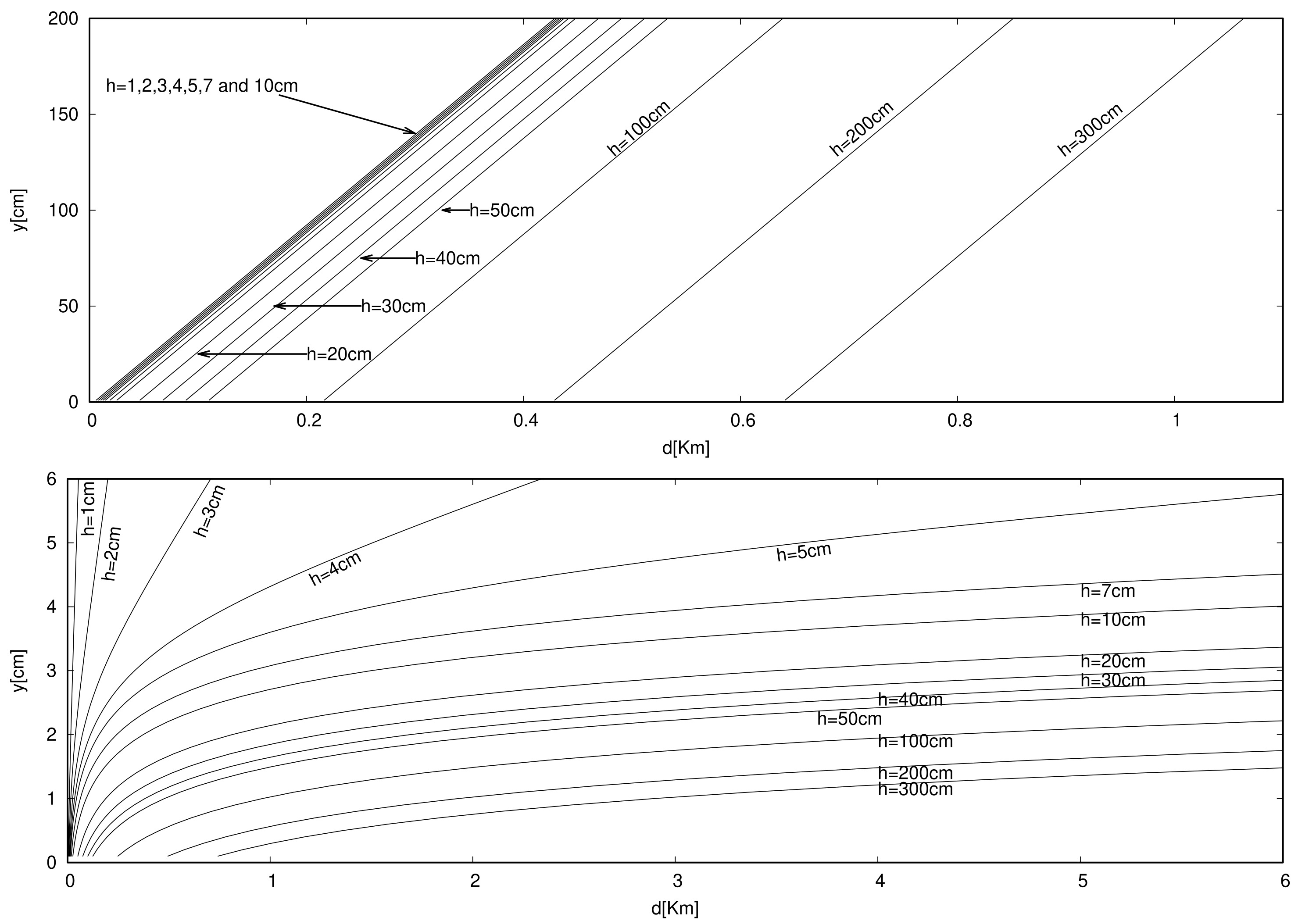
FIGURE 6 Minimum distance (curve L3) and invisibility limit (curve L4) for seeing an inferior mirage, in panels a and b, respectively, for point object at different heights. 

It is obvious that in real life situations the objects are not generally point-like but vertically extended from the ground. Interesting conclusions can be reached from the results shown in Fig. 6 for these cases. Since the minimum distance to see the mirage increases with h, it is possible that the observer sees the image of the lower part of the extended object, but not the image of its upper part. For example, under the meteorological conditions considered, the observers would not be able to see the image of the upper portion of a palm tree above 2 m, if they are at 745 m from it with their eyes 1.5 m above the ground. On the other hand, due to the existence of a region of invisibility, it is possible the opposite situation, producing a discontinuity between the object and its image that would make observers to experience the impression that the object is floating. For example, observers located 3 km from the palm tree would not observe the 2 cm closest to the ground or its image, if their eyes were lower than 70 cm from the ground. It is worth mentioning that this impossibility of observing the base of objects and their images from certain positions has nothing to do with a similar effect caused by the variation of the distance to the horizon with height due to the sphericity of the Earth (for example, when the base of the ships disappears under the horizon before the sails), which is not considered in this work.

Finally, we analyze how atmospheric conditions influence the delimitation of the identified regions. To do this, we calculated the curves L1, L2, L3 and L4 for a point object at a height h = 5 cm and different temperature profiles (expressed in terms of different values of α and β). The results are displayed in Fig. 7 for appropriately selected cases (which were previously indicated in Fig. 1). Note that all cases, except 3, correspond to T ₁ /T ₀ ratios close to those selected to build Fig. 1. For case 3 T ₁ /T ₀ = 0.37, which represents a very abrupt drop in temperature in the first centimeters of atmosphere. It jumps out from Fig. 7 that, as the values of α and β increase, the limits of the different regions approach each other, progressively turning to the ordinate-axis. For higher temperature conditions (greater α and β values), the regions where it is possible to see only the object or only the image become smaller (being appreciable only near the point object), and the region where it is not possible to visualize the object nor its image is enlarged. For example, while in the reference case the observers located 4 km from a point object should have their eyes lower than 5 cm above the ground for not seeing the part of the object below 5 cm or its image, under more extreme weather conditions, the observers could have their eyes 50 cm above the ground and experience the effect. Thus, we can conclude that for both, large h values and large α and β values (being the effect more pronounced when β increases) the differentiation on four types of regions become less evident, tending to only two: above L4, where object and images would be seen, and below, where neither would be seen. In the opposite case, for very small α and β values, the region where the object and its image could be seen enlarge considerably, so that the region delimited by the curves L1, L2 and L4 (where only the image could be observed) becomes very small and tends to disappear for reasonable distances to the object. In all cases, the region where only the image can be seen is reduced for reasonable observer distances. Hence, although possible, it is unlikely that an observer would see only the image of an object.

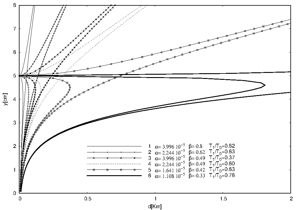
FIGURE 7 Visualization regions of a point object or its image, delimited by curves L1, L2, L3 and L4, for different α and β values. The selected cases have been identified in Fig. 1. 

5. Conclusions

In the present work we analyze the locations of potential observers appropriate to see an object and/or its image, applying the method for calculating ray trajectories on the occasion of inferior mirages presented in Ref. [¹⁰]. The expression found to describe the path of each ray allows to distinguish its descending part from its ascending part, by locating the point of maximum approach of the ray to the ground (V point). We have analytically verified that the V points of the rays, emerging all of them from a point object, progressively move away from it until they reach a maximum distance, after which they approach the point object again. This maximum distance achieved undergoes a pronounced increase for small increases in the height of the point object.

The curve that joins the V points of all the rays emerging from a point object represents one of the limits of the region in which only the inverted image of the object can be observed, since the visualization of isolated images only occurs in regions of space where there is no descending part of rays. The first ray that does not present a descending part, and the lower envelope of the ray paths constitute the other limits. The latter is also a limit for the visibility of the object, since below this line, any observer would not receive neither direct nor refracted ray. Finally, an additional limit arises by considering the first ray that, emerging from the point object, is not absorbed by the ground, so that, for smaller distances than the ones represented by this line, observers receive only direct rays. All these limits (which we have named curves L1, L2, L3 and L4) have analytical expressions that reproduce them, so they can be represented for any atmospheric situation and any object position.

Finally, we have analyzed the influence of atmospheric conditions on the delimitation of the observation regions of the phenomenon. All the curves are expressed in terms of two parameters, α and β, which can be determined from the measurement of the air temperature at three different heights (surface, 1 cm, and field). Although from different temperature profiles the same α and β values can arise, we can assume that, in general, both parameters increase as the thermal amplitude between the soil and the field increases. From our calculations for different α and β values we observed that, as one or both parameters grow, the different visualization regions of object and/or images become smaller, while the invisibility zone is enlarged. If, in addition to large values of α and β, we consider higher objects, the regions tend to reduce to two: one where the object and its image are seen, and another where none of them are seen.

Analytical determination of visualization regions may have practical implications. On the one hand, if we know the atmospheric conditions it is possible to predict where an observer should be located to see the inferior mirage in a particular way. On the other hand, the observation of the phenomenon could be used to infer the temperature profile near the ground. To complement this series of works, and having already characterized the different visions of the inferior mirages that a casual observer could experience, in the next study we will explore the location of the images according to the observer and the object locations.