


 nueva página del texto (beta)
 Inglés (pdf)
 Artículo en XML
 Referencias del artículo
 Enviar artículo por email
 Citado por SciELO
  Similares en
SciELO
Similares en
SciELO 
 Permalink
1. Introduction
Helical segmented-fin or serrated-fin tubes are widely used in heat exchangers because the heat transfer surface decreases, and consequently, the weight of the thermal equipment is reduced. The heat transfer performance is not sacrificed because the geometry of finned tubes promotes turbulence, although the pressure drop also increases. In the open literature, experiments and numerical simulations have studied the thermal-hydraulic behavior of helical segmented-fin (serrated-fin) tubes. Most experiments present global studies of heat transfer and pressure drop on finned tube banks [15]. Some works compare the thermal performance of different serrated-fin geometries, as developed by Zhou et al. [1]. Other studies analyze the effect of segmented-fin (serratedfin) characteristics, such as fin pitch, fin height, fin density, and segmented fin height on heat transfer and pressure drop. For instance, heat transfer and pressure drop increase as fin height and fin density increase, as reported by Naess [2] and Ma et al. [3]. In contrast, the fin pitch has a reverse behavior because heat transfer and pressure drop decrease, as found in Naess [2] and Kiatpachai [4]. Keawkamrop et al. [5] found that segmented fin height significantly affects the Nusselt number. Some experiments report detailed information as visualizations [6, 7] and velocity measurements [8]. For example, Pis’mennyi [6,7] identified experimentally intense vortical structures in the front of the fins, which increased the transfer of momentum and energy. Papa [8] measured the velocity field and turbulence parameters in half of a finned tube.
On the other hand, numerical simulations present detailed information on the heat transfer performance of a singlefinned tube [9-13] or a small-finned tube bundle [1,14-22]. Most numerical simulations focus on representing the flow around the finned tube and its connection to heat transfer [1,9-11,14,15,17,18,20,21]. For example, Martinez-Espinosa et al. [18] found intense temperature gradients near the vertex of segmented fins where heat transfer is intense. Other investigations included parametric studies of fin characteristics (segmented fin height, fin pitch, fin height, or fin thickness) on heat transfer [12,13,16,19]. Anoop et al. [12] found that segmented fin height has the same thermal performance as plain fins, with less heat transfer area. Finally, few works have studied the turbulent structures in helical segmented-fin tubes and their relation to energy transport. Kumar et al. [19] found vortices generated by fins and horseshoe vortices along the tube surface that enhanced the heat transfer. These vortices were identified through vector maps and streamlines in a RANS) simulation (Reynold Average Navier Stokes). Salinas-Vázquez et al. [22] found relevant momentum transfer in the inter-segment space, which increased the turbulence and the formation of vortices between the fins at high spaces between the segments.
State-of-the-art research reveals that few works have studied turbulent structures in helical segmented-fin tubes [19, 22]. Studies of heat transfer performance reveal that heat transfer is intense in the vertex of segmented fins [5,18] and influenced by the presence of vortices in these zones [6]. Few studies have been conducted on turbulence structures and their connection to heat transfer and pressure drop in helical segmented-fin tubes. Therefore, this study continues the turbulence study developed by Salinas-Vázquez et al. [22] while considering studies on the vertex of segmented fins conducted by Martinez-Espinosa et al. [18] and Keawkamrop et al. [5]. The primary objective is to propose a way to increase the thermal performance of helical segmented fins without an increase in pressure drop and heat transfer surface. Then, a numerical study of the anisotropic state of the turbulence is developed at different segmented fin heights. Simulations were conducted using the large eddy simulation (LES) approach and numerical tools, such as periodic boundary conditions and the immersed boundary technique. Four cases were simulated at different segmented fin heights to understand the effect of the depth of the fin segmentation on thermal-hydraulic performance.
2. Governing equations
The compressible Navier-Stokes equations in a Cartesian frame of reference can be written as follows [23]:
where U is the vector of conservative variables, defined as:
where u i represents the velocity component in the i−direction, and ρ is the density. In the results section, both the velocity and space direction vectors were changed from (u 1 ,u 2 ,u 3) to (u,v,w) and (x 1 ,x 2 ,x 3) to (x,y,z), respectively. The total energy, which is the sum of internal and kinetic energies, is defined for an ideal gas as follows:
F i is the fluxes in the three spatial directions.
where k is thermal conductivity, δ ij is the Kronecker delta, and S ij is the deformation tensor, defined as:
The vector S F , corresponding to the source terms, is a function of time only and is necessary to counteract the friction losses in the principal direction. Force must be introduced to represent a fully-developed flow economically (Fig. 1a) by imposing a constant mass flux in the periodic main flow direction. This forcing term, f s (t), is equivalent to the imposition of a mean streamwise pressure gradient (see the appendix in Salinas et al. [22]). The forcing appears in the energy equation multiplied by the mean bulk velocity Eq. (7).
3. Numerical solution
3.1 Numerical scheme
Equations (1) to (4) in the generalized coordinates were solved using the fully explicit McCormack scheme [24], second order in time, and fourth order in space.
3.2 Initial and boundary conditions
The thermodynamic variables, temperature, and pressure (or density) were initialized by a constant value and equal to their reference values of T ref and P ref (atmospheric conditions). The tube temperature is constant through the simulation and equal to T tube = 1.4T ref . The streamwise velocity (x−direction) was equal to its reference value of U 0 = U b , which was the bulk flow velocity in the domain, defined as:
The mean bulk value of a variable is given by:
where
Two spanwise velocity components (y−z
direction) were considered null (V
0 = 0 and W
0 = 0). Periodic boundary conditions were applied in the
x− and y−directions. Physically, this
implied that the lateral walls did not influence any of the two directions. This
condition consists of cloning the computation domain in the periodic directions,
see Fig. 1a). This boundary condition
allows the simulation of an infinity of tubes at the fully developed zone of the
tube bundle (after four to five rows of the inlet and far from the lateral walls
[25]) while saving computer
resources. A forcing term (Eq. (6)) must be imposed to prevent the flow stop and
the creation of the pressure drop, a non-periodic condition (see Appendix in
Ref. [22]). Slip walls [26] were imposed in the z-direction. The
boundary condition is based on the method called Navier Stokes characteristic
boundary conditions. The hyperbolic terms of equations are modified at the
boundary by characteristic analysis in the form of waves normal to the boundary.
For slip wall, an invisid conditions is imposed at the wall:
3.3 Turbulence model
The turbulent effects were simulated with a LES model. According to Metais and Lesieur [27, 28], small scales should be filtered, and their effects included in the present model through the classic eddy-viscosity assumption, (ν t ). The subgrid-scale model used in this work is the selective structure-function model proposed by [29]. The local eddy viscosity, ν t (x,t), is then given by:
where C ssf is expressed as a function of the Kolmogorov constant C k , C ssf = 0.104. Local filter size, ∆, is taken equal to (∆x∆y∆z) 1/3 , where ∆x, ∆y, and ∆z are the local grid sizes in the three spatial directions. F 2(x,t), the second-order velocity structure function constructed with the instantaneous filtered field. F 2(x,t) is calculated at a given point with a local statistical average of square (Favre-filtered) velocity differences between the given point and the six closest points surrounding the computational grid.
3.4 Immersed boundary conditions
Immersed boundaries allow solid bodies with complex geometries to be introduced into the flow. The complex solid body geometry of the fins was generated using computeraided design software in STL format (Standard Triangle Language) and transferred to the computational domain (own numerical tool).
To identify the solid, we used a level set function, ϕ(x), which took the value of −α inside the solid and +α outside the solid. α is proportional to the maximum grid size in the computational domain [22,30, 31]. Ghost nodes were identified as those nodes that are close to the solid body without being part of it(see Fig. 2a).
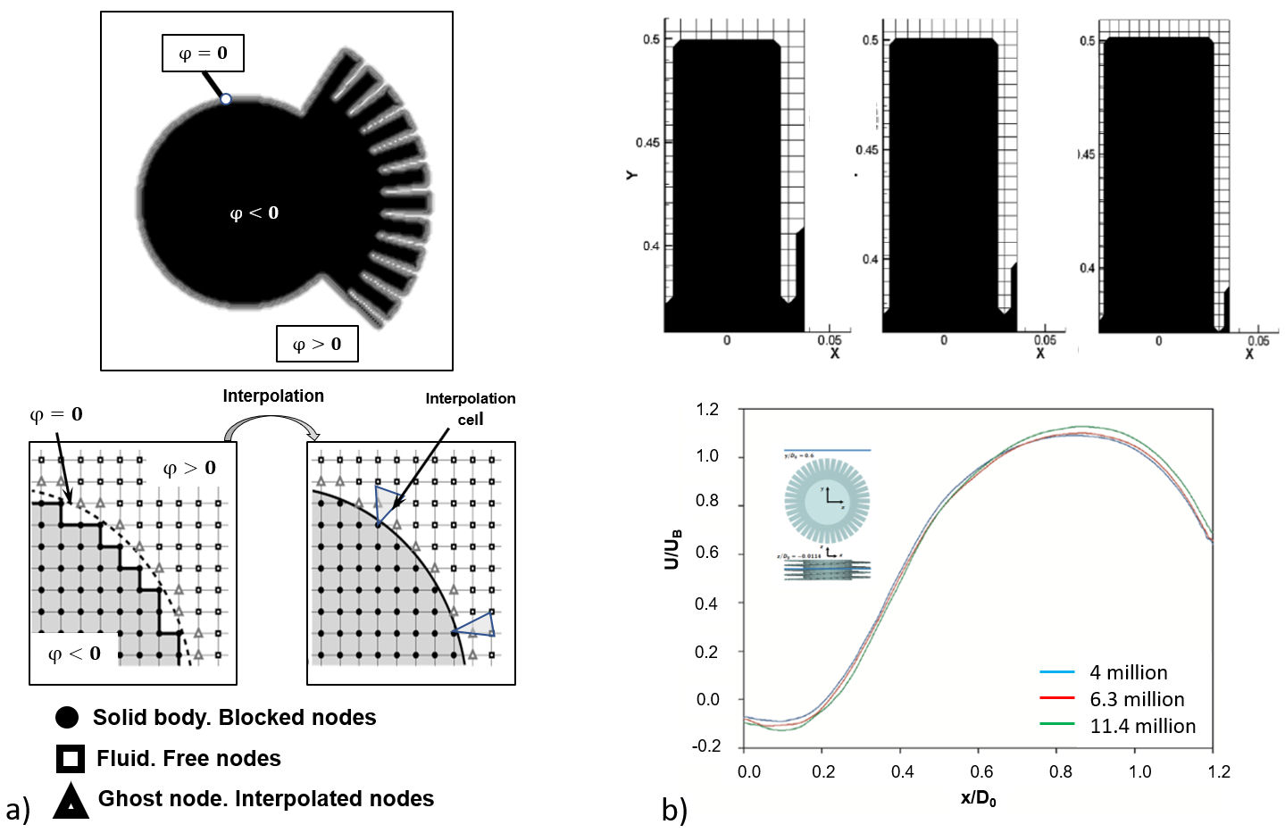
FIGURE 2 Immersed boundary conditions and grid independence. a) Immersed boundary conditions based in the use of a level set function ϕ. Interpolation of the solid body variable values avoids the stepping behavior. b) Fin representation in three different grid resolutions. Mean streamwise velocity comparison for three different grid resolutions.
After a reinitialization process of the level set function [30,31] to keep ϕ(x) as a signed distance function. The solid surface was obtained with good precision at the zero-level of this function (ϕ(x) = 0). The solid body was created by imposing harsh conditions, such as null velocities and a constant temperature, at the blocked nodes (ϕ(x) < 0, see Fig. 2). The velocity at the ghost points was interpolated (linear 2d and 3d interpolations) from the values of their nearest neighbor nodes. This procedure avoided a stepping behavior of the velocity field close to the walls; the complete procedure can be seen in [32]. The pressure was extrapolated from the fluid to the solid [33], which allowed for a null pressure gradient at any wall surface, ∂p/∂n| wall = 0. The extrapolation was obtained from the following advection equation:
where n is the normal to the wall unit at every grid point, defined from the level set function, ϕ as:
where τ is not the physical time, but a function of the grid τ ∝ min(∆x∆y∆z). Five time steps were required to populate the needed nodes. Advection equation Eq. (10) was solved using a third-order total variation diminishing (TVD) Runge-Kutta scheme for time discretization and a fifth-order weighted essentially non-oscillatory (WENO) scheme for space discretization [34]. The extrapolation procedure was done for every time step of physical time, t.
4. Validation
The validation was conducted in two stages. In the first, the numerical and experimental results obtained by Simonin and Barcouda [25] were compared in a smooth tube bundle [32]. In the second stage [22], the mean streamwise velocity was compared with the experimental results [8].
5. Simulation characteristics
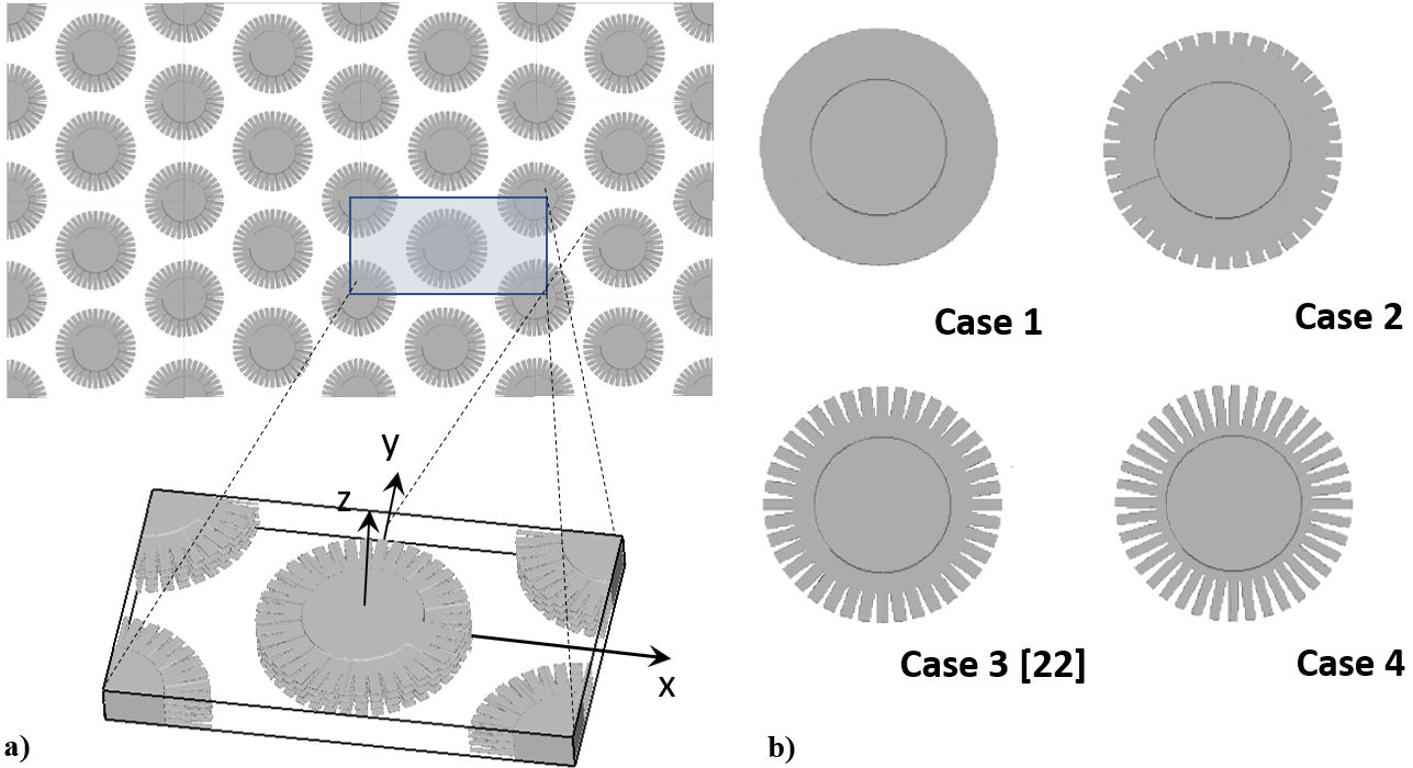
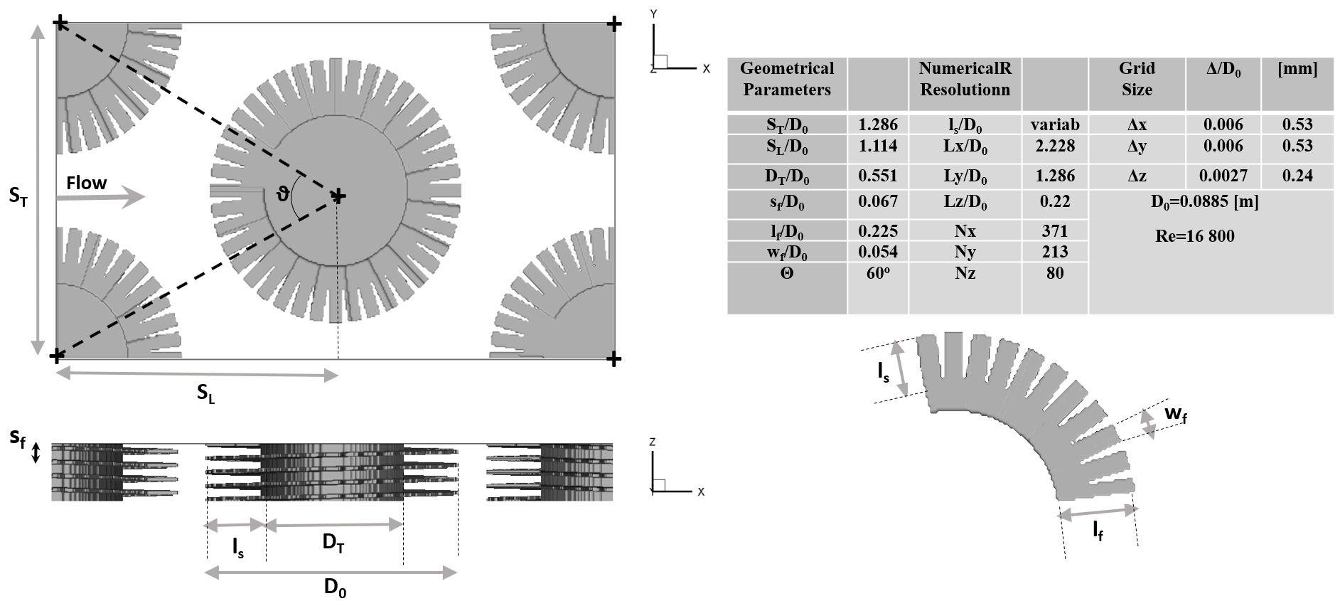
The computational domain was the same as in a previous study [22]. The reduced domain comprised a complete tube at the center and four quarters in the corners (see Fig. 2). In this work, only the hydrodynamics of the fluid were studied. The Reynolds number (Re = (U b D 0 ρ ref )/(µ(T ref ))) used in this study was 16890 (equal to that used in Martinez et al. [18] and Salinas-Vázquez et al. [22]. The dimensionless computational domain lengths are (D 0 = 0.0508 m): 2.228D 0 × 1.286D 0 × 0.22D 0 for the x−, y−, and z−directions, respectively. Due to the complexity of the tubes, the grid was uniform in all three directions. The grid resolution is 371×213×80 computational nodes for the x−, y− and z−directions.
This resolution was obtained after studying the independence between the grid resolution and the results [35]. For this flow, the main difficulty was correctly capturing the geometry of the fins. In Fig. 2b), we show the fin resolution for three different cases (4,6.3, and 11.4 million computational nodes). We found that for resolutions 50% lower than the one used here, significant changes (2−3%) were not observed in the statistical results. Figure 2b) shows the comparison of the mean streamwise velocity in a given position. The same behavior was observed in mean and turbulence quantities.
In engineering, the best solutions are the simplest. For this reason, the present work intends to complement previous works [22] on the subject by changing the fin segmentation depth, l s . Four different configurations [Fig. 1b)] were studied: l s /l f = 0.0 (smooth fin), 0.25, 0.5 (base case [22]), and 0.75, where l f is the total fin length and l s is the segmentation depth [see Figs. 1b) and 2b)]. The flow characteristics, computational domain length, and resolution were the same for all cases (Fig. 3).
5.1 Statistical variables
We define the mean quantities as the average of the variable across time. For any
given instantaneous quantity
where
The second and third invariants of the tensor are defined as [36]:
Based on the previous invariants, the η and ξ variables are defined as [36-38]:
The anisotropic state of turbulence can be described by a characteristic spheroid whose radii correspond to the eigenvalues [37]. The anisotropic state of turbulence parameter [F] scales the degree of anisotropy from zero (one-or twocomponent turbulence, anisotropy) to one (isotropic turbulence), and it is defined as [36-38]:
6. Results
6.1. Mean streamwise velocity
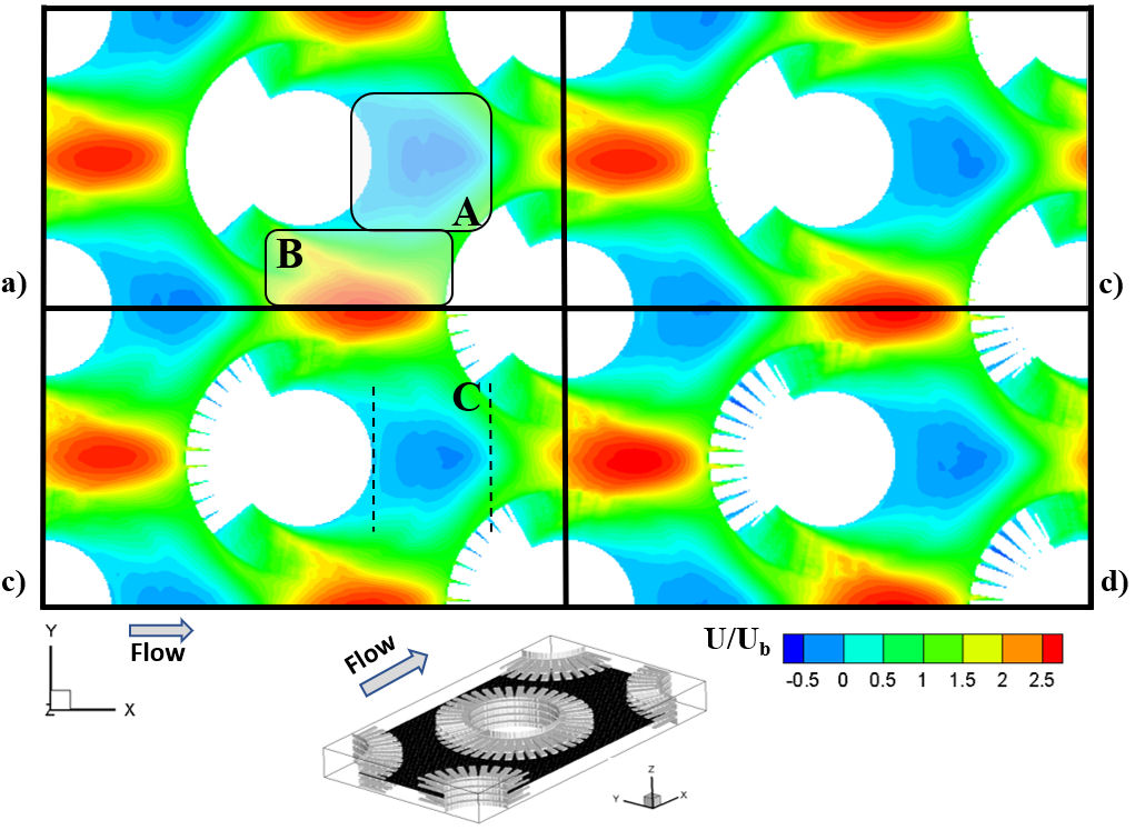
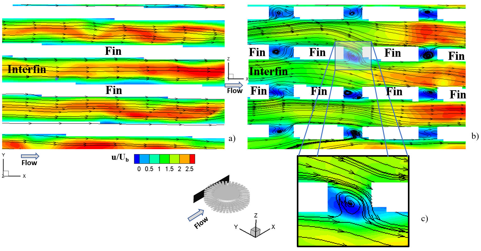
Figure 4 shows the mean streamwise velocity in a z-plan. The darker blue zones (negative velocity values) show recirculation zones. As seen in previous works [22], the mean velocity field shows a pair of symmetrical recirculations behind the tubes (dark blue zones, A-square) and high-velocity bands away from the tubes (red zones, B-square). However, several antisymmetric recirculations were observed in instantaneous fields [22]. Recirculation size (C-lines) and the minimal and maximal mean streamwise velocity values were similar for all cases studied. A comparable situation was observed for the other components. Small changes in velocity fields bring with them minimal changes in pressure drop. A great advantage in heat exchanger design is the marginal increase of < 2% in the pressure drop observed between Cases 1 and 4.
6.2. Interfin zone interactions
The main change in the flow for the different cases studied was found in the interfin zones. The interaction between these zones is shown from instantaneous velocity fields. Figure 5 shows the trajectory lines in the y-plane. The flow goes from one zone to another through the spaces made by the fin segmentation (Fig. 5c). The instantaneous and mean magnitude of the normal velocity component increases in this zone.
6.3. Turbulence intensities
Figure 6 shows the turbulence intensities
(rms-values) and the turbulence kinetic energy
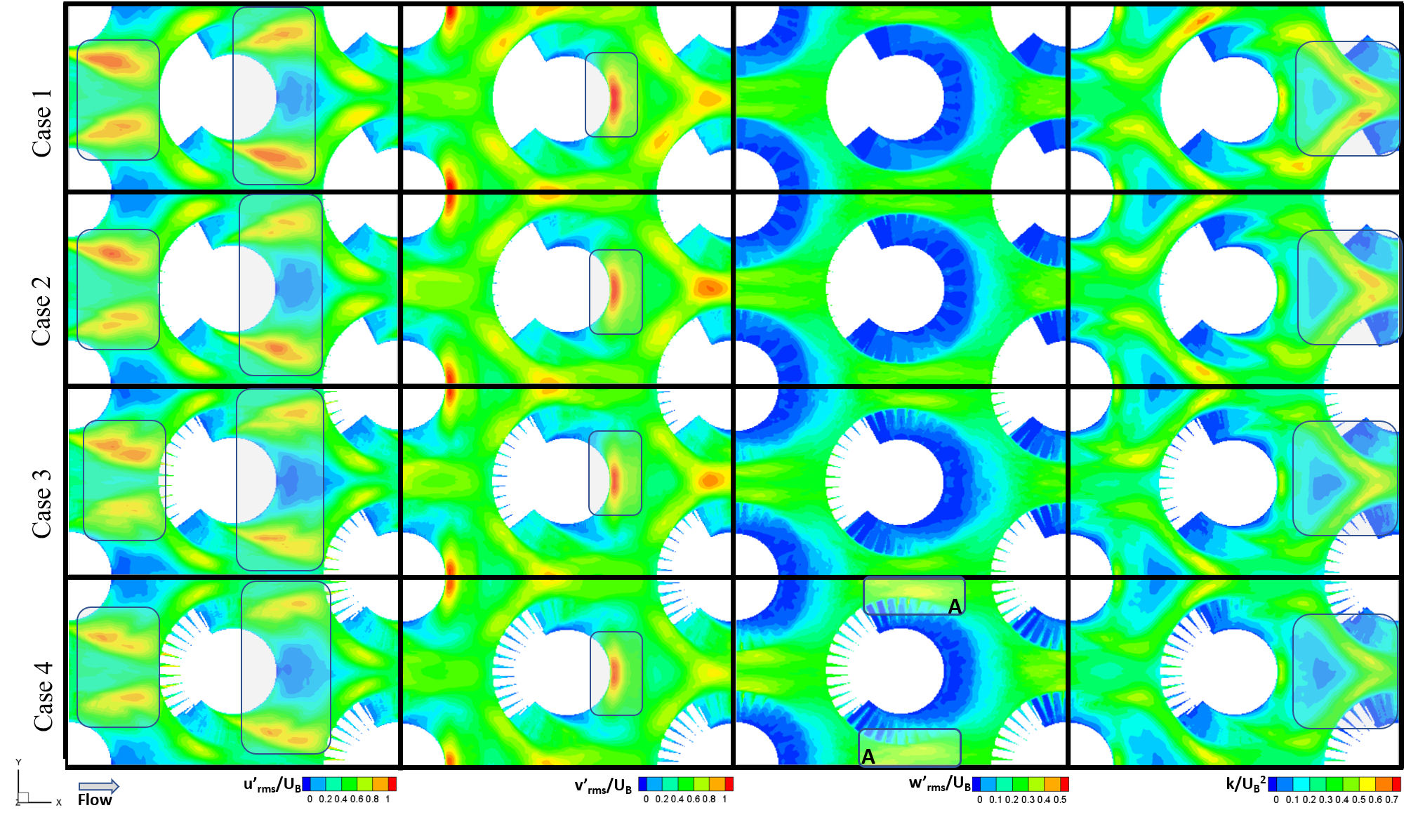
FIGURE 6 Turbulence intensities
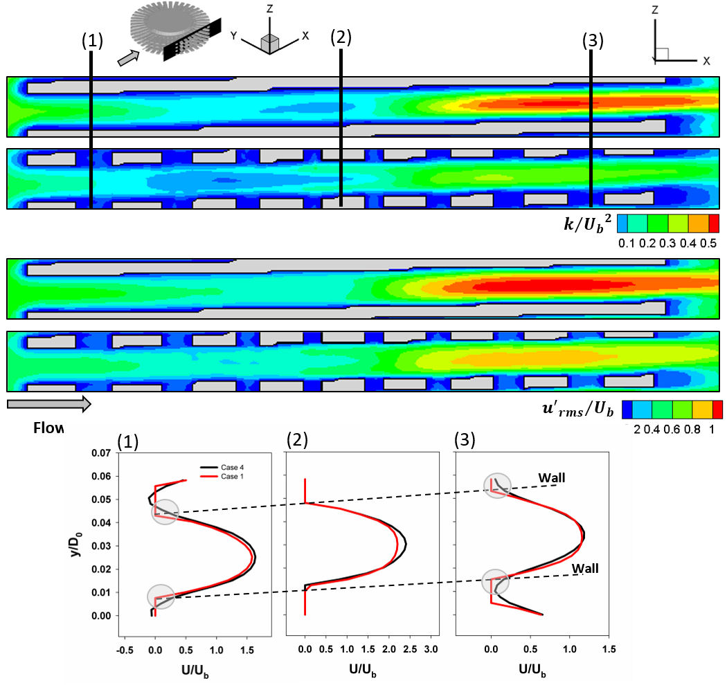
FIGURE 7 Turbulence intensities
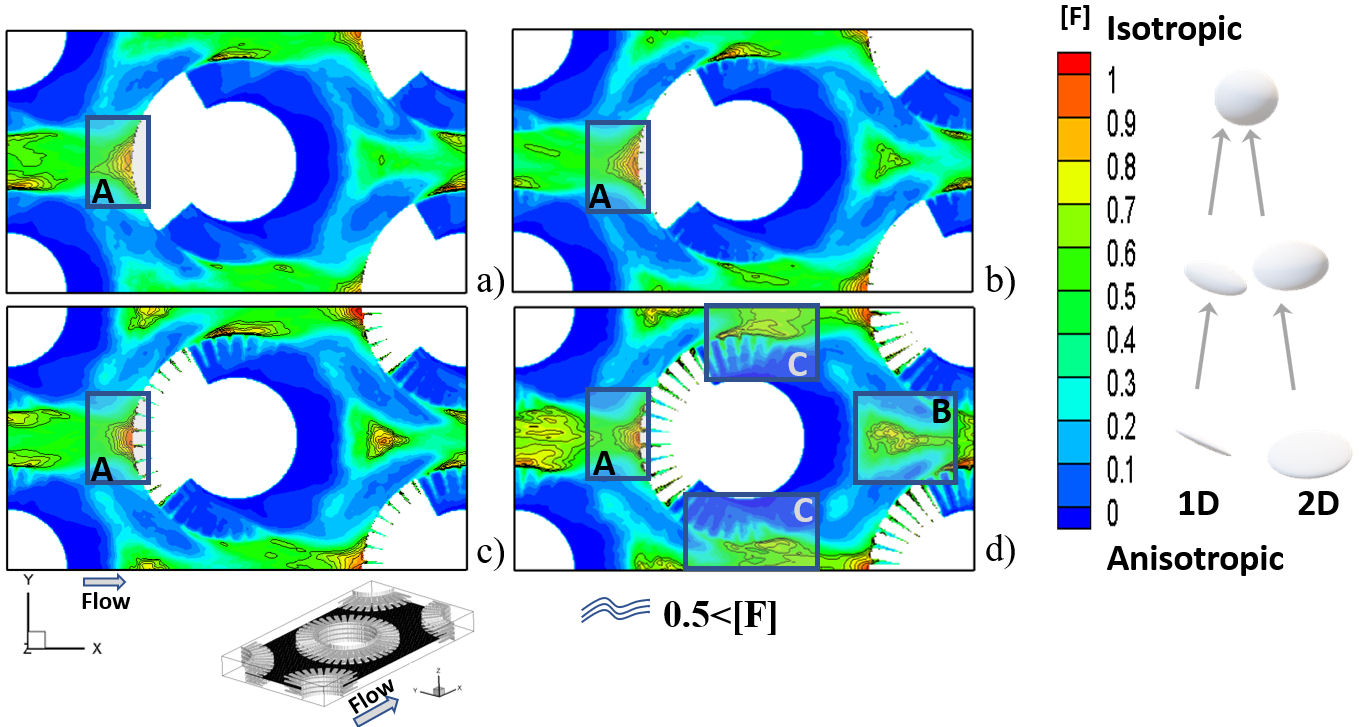
FIGURE 8 The anisotropic state of turbulence parameter [F] contour in a z-plane, z/D 0 = 0.1; a) Case 1, b) Case 2, c) Case 3, and d) Case 4. Line contours show 0.5 < [F] zones.
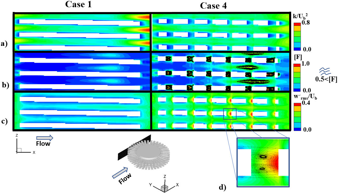
FIGURE 9 Turbulent variables in a y-plane,
y/D
0 = 0.44, include a) turbulence
kinematic energy, k, b) the anisotropic state of
turbulence parameter [F], c) turbulence intensity,
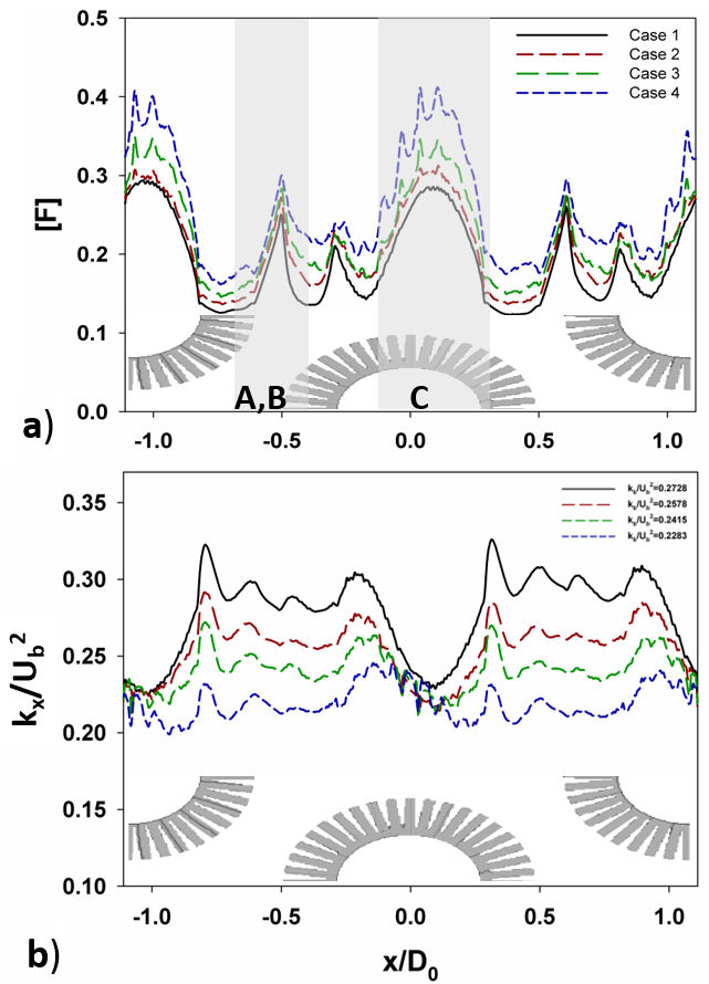
FIGURE 10 Streamwise mean profiles: a) [F] parameter (A-,
B-, C-squares in Fig. 8), and b) turbulence kinetic energy,
To understand better the turbulence decreases, see Fig. 7. The wall turbulence feeds on the velocity gradients
generated near the wall. When the flow touches the fins and the tubes, the
boundary layer develops generating turbulence. If the wall is discontinuous,
case 4, the boundary layer development is weak and the turbulence in the flow is
lower. Figure 7 shows the
Despite the previous changes observed in the magnitude of the turbulence
intensities outside the fin zones, the anisotropic state of turbulence is also
transformed. The turbulence in this flow was highly anisotropic because it has a
preferential flow direction (streamwise direction). This flow changed direction
around the tubes and transfer turbulence energy from the streamwise (
However, the fins restrict the transfer of turbulence energy to the third
direction,
Figure 9 shows the contours of the three
turbulence variables in the y-plane. In this zone, an increase
in the component
Figure 10 shows the streamwise mean profiles of the [F] parameter and the turbulence kinetic energy k. The values were obtained from a variation of Eq. (8), integrated only in the y − z planes:
where A(y − z)Free Total are the free yz-area of every xplane. The important thing to highlight is the areas where the variables are the maximum. In the case of parameter [F], the maximum value was observed in front of the tubes A-square (Figs. 8 and 10) behind the tubes (B-square) and on the sides of the tubes, generated mainly by the separation of the boundary layers C-square (Figs. 8 and 10). Figure 10a) shows a third peak at the beginning of the last zone mentioned above. The small peaks in Fig. 10a) (in the C- squares) are the effect of fin segmentation. The streamwise mean maximum values for Case 4 are [F] ≈0.4, and for Case 1, [F] ≈ 0.28. However, locally, the value can reach close to 0.9 for all cases. See square A in front of the central tube in Fig. 8. For turbulence kinetic energy, the distribution was more uniform. The variable decreased around the tube center. The highest streamwise velocity was observed in this zone (Fig. 4). In this zone, the minimum values of the fluctuations of the principal components are found. However, an increase in the third component, A-square (Fig. 6), was observed for Cases 3 and 4. Figure 10b) shows the bulk mean Eq. (8) values for each case. A maximum decrease of 16% was found between Cases 1 and 4.
7. Conclusions
This study analyzed the effect of fin segmentation depth on turbulence in a helical fin tube bundle. Much of the turbulence generated is due primarily to the boundary layers and the wakes behind the solid bodies. In the case of segmented fins, the discontinuity of fin walls does not allow the complete development of boundary layers, obtaining a reduced turbulence kinetic energy (Fig. 10) of up to 15% in Case 4 compared to Case 1. Despite the decrease in the magnitude of the turbulence, the fin segmentation generated a state of turbulence closer to isotropy, which would transform heat transfer (this work is in progress). This assumption is based on the turbulence transformation observed in the interfin zone, where heat transfer was produced in this flow. Likewise, an intense flow interaction was observed between interfin zones.

