1 Introduction

Tropospheric ozone (O₃) is formed from the chemical reaction between the action of sunlight and different precursor substances such as volatile organic compounds, carbon monoxide (CO) and nitrogen oxides, among others studied by ^[1]; it has origin in combustion processes from industrial emissions and vehicular traffic defined by ^[2]. Given the nature of O₃ in large cities, it is subject of numerous studies that show its adverse effects on health ^[3-5]. For this reason, studies of the temporal records of O₃ have been carried out to understand its behavior from data analysis ^[6,7]. Also, it have been found the climatic variables play an important role in the process of accumulation or dispersion of O₃ concentration levels ^[8,9]. For example, in the Klang Valley, Malaysia between January 1997 and December 2006, the analysis show that the concentrations of some pollutants, such as CO, NO₂ and SO₂, are higher in the stations that report the heaviest traffic and the concentrations of PM₁₀ and O₃ are influenced by regional tropical factors, biomass burning, and ultraviolet radiation ^[10]; furthermore, they considered significant differences between pollutant concentrations in different monitoring stations, suggesting that the local environment influences the concentration of gases in each season. In similar way, in Malaysia during period from 1999 to 2010, it were reported in their study variations in O₃ levels due to meteorological variables with highest concentrations in the first quarter of 2009 ^[11]. Also, they show that the average O₃ concentration was higher in February and lower in November.

The evaluation of O₃ contaminants carried out by ^[12], in Deradun, India, consider environmental volatile organic compounds (VOC) samples for three seasons: summer, winter and the monsoon. They report that recorded toluene environmental concentration is higher during winters and lower in monsoons. According to ^[12], the high toluene proportion indicates vehicular emission as the main source, because toluene and xylenes are found in the hydrocarbons that contribute the most to O₃ formation ^[13], in the city of Tenerife, describe the influence of climatic conditions and find that the PM₁₀ are lower during the rain and describe the temporal evolution of the pollutant concentrations, O₃ included.

On the other hand, the findings in the literature suggest several underlying relationships between meteorology, anthropogenic sources, and pollutant concentrations that are useful for establishing local trends in air pollution over time and geographical space. Hence, a large number of researchers have focused their efforts on characterizing O₃ contamination records among others ^[14-17]. To accomplish this, they make use of Fractal theory tools due to the complex and chaotic nature of the phenomenon. Consequently, it has been possible to characterize data series of different environmental pollutants with a small data set.

This paper is structured as follows. In Sec. 2, state of the art review on statistical persistence studies of air pollutant records in different cities in the world are considered. Section 3 describes the performed analysis using seasonal fluctuation and structure function to that characterize long-term correlations of the data series. Section 4 shows the results obtained to explain the behavior of the data series for the different seasons of the year in Mexico City. Finally, in Sec. 5, conclusions are described.

2 State of the art review

In the last decades, studies have been conducted on the statistical persistence in air pollutant records in different cities around the world ^[18-23]. It was also established that time series associated with different air pollutants are complex systems and multifractal in nature ^[24-28]. The multifractal behavior was characterized under different analysis metrics, from those referred to as FA fluctuation analysis, FDA detrended fluctuation analysis, rescaled range, spectral analysis, two-dimensional multifractal detrended fluctuation analysis (2D-MFDMA) ^{[18,26,27,29]}. A study on air quality index (AQI) time series for CO, NO₂, O₃, PM_2.5, PM₁₀ and SO₂ pollutants using multifractal fluctuation detrended analysis (MF-FDA) was carried out by ^[28]; He found multifractal behaviors for pollutant concentration series for Beijing, Jinan and Zhengzhou cities in China. In other study conducted on API time series between 2001 and 2012 in Nanjing, China, the multifractal nature and long-term correlations were reported by ^[25]. Furthermore, the existence of multifractal nature and statistical persistence, i.e., long-range correlations, for major air pollutants O₃, SO₂, CO, NO₂, and PM₁₀, in Mexico City, have also been empirically demonstrated, as can be seen in ^[20,24]. On the other hand, analysis on atmospheric pollutants from a classical fractal model and the fluctuation associated with these series of records were conducted on other works. For example, during the period 1993-1999, studies of pollutants O₃, PM₁₀ and PM₂, using Sigma-T (ST), Hurst and the rescaled range to determine the Hurst exponent index were carried out in the United Kingdom by ^[30]. They found persistence of pollutant fluctuation over a temporal period of days. Detrended fluctuation analysis (DFA) on time series of O₃, NO_X and PM₁₀, for the cities of Athens, Greece and Baltimore, USA, were performed by C.A. Varotos, et al., ^[30]. They found that while O₃ and NO_X pollutants show persistance in time scales ranging from one week to five years; for PM ₁₀ persistence appears at intervals of four hours to nine months. Also, the Detrended MovingMedian (DMM) method to estimate both the Hurst persistence degree and persistence properties of ozone concentrations, from eight air quality monitoring stations in urban and suburban areas of peninsular Malaysia, was used by ^[32]. The previous studies empirically determine the multifractal condition of the time series of atmospheric pollutants in different cities of the world, including Mexico City; as well as the persistence associated with the time scale. In addition to this, other works report the influence of both meteorological factors, i.e., temperature, humidity and wind speed ^[26]; and seasonal effects, on concentration levels through long-term correlations ^[18]. However, as it is well known, quantitatively the formation, deposition and distribution of pollutants in the environment are characteristic of the dynamics of environmental factors and anthropogenic activities in each region of the world ^[33-35]. Then, it is important to understand the extrinsic information of the factors influencing the time series behavior of various atmospheric pollutants with respect to seasonal dynamics. For this reason, a local analysis is proposed to examine the statistical persistence associated with the time scale of the influence of meteorological factors implicitly associated with the dynamics of each season of the year.

In this work we use a metric that determines the characteristic behavior of time series (in the context of the Hurst exponent), in particular those associated with O₃ records from four different RAMA sites in Mexico City. Consequently, a quantitative estimation of the statistical behaviors of persistence, antipersistence and randomness of the spring, summer, autumn and winter seasons of each year analyzed is given.

3 Methodology

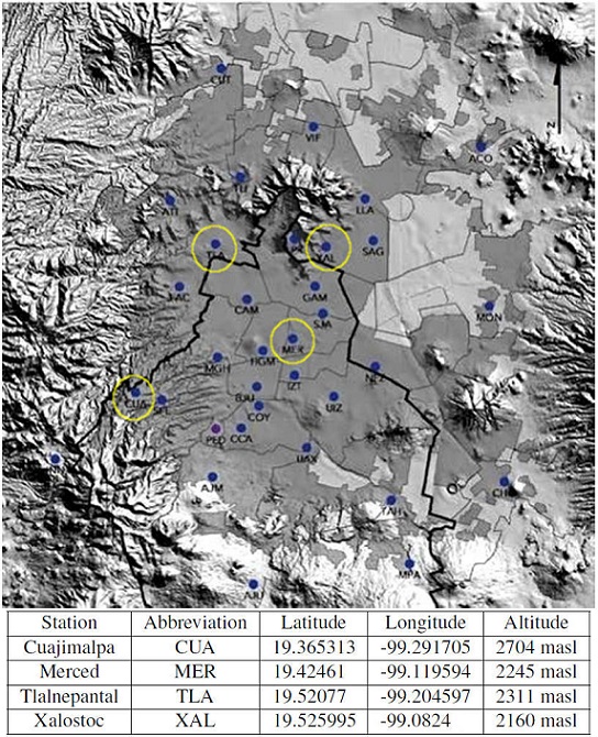
We analyze the fluctuations of the time series associated with O₃ in Mexico City during 2010-2018, and determining the persistence in the seasonal periods, i.e., Spring, Summer, Autumn, and Winter, through the dynamic scaling approach using the structure function ^[36]. In this work, the used records of O₃ concentration indices were obtained from Automatic Atmospheric Monitoring Network (AAMN) of Mexico City from four different monitoring stations: Cuajimalpa (CUA), Merced (MER), Tlalnepantla (TLA), and Xalostoc (XAL), according to Fig. 1. The concentration indices correspond to a nine-year period, from 2010 to 2018, and time series are constructed from data of the seasonal periods Spring, Summer, Autumn, and Winter. The persistence of these seasonal periods is studied by determining the Hurst exponent (H) for the fluctuation associated with these time series by means of the second order structure function.

Figure 1 Location of air quality monitoring stations in Mexico City. 

3.1 Data collection

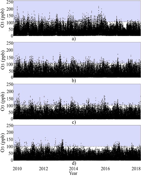
The Atmospheric Monitoring System (AMS) of Mexico City is responsible for the permanent measurement of the main air pollutants (SO₂, NO₂, CO, O₃, PM₁₀, and PM_2.5), AAMN is made up of 29 monitoring stations and provides immediate information for activation or deactivation of alert or emergency procedures for environmental contingency. In addition, it has historical records of the pollutants of Mexico City and the metropolitan area (http://www.aire.cdmx.gob.mx/default.php). Hence, the daily records by hour of O₃ from January 1, 2010 to December 31, 2018 of the CUA, MER, TLA, and XAL monitoring stations are considered. Figure 2 shows the total records from each site with their respective concentration variation in parts per billion (ppb).

Figure 2 O₃ concentration profiles of four monitoring stations: a) CUA, b) MER, c) TLA and d) XAL. 

The following data for each monitoring station are considered: 56217 records were taken from CUA, 56239 records from MER, 54744 records were 140 taken from TLA and 58687 records from XAL. In general, there are 9 years of records corresponding to four monitoring sites, for a total of 36 samples for each season of the year (see Table I). Notice the data differences of the consulted records, this is because in some hours the monitoring station were in maintenance or calibration (See Table I). Each site was chosen because they manifest highest levels of O₃ in Mexico City. For example, XAL corresponds to an area composed of a high vehicular traffic that connects the Metropolitan area in the northern part of Mexico City, and every day around 1.5 million people mobilize to carry out their work and education activities. In addition, it has an industrial zone, that is considered one of the most polluted areas in Mexico. TLA is another area that is immersed in the Valley of Mexico and it is part of the most polluted places in the country providing 18% of greenhouse gases. MER is in the center of Mexico City with commercial and vehicular traffic activities. CUA is in the southwest of Mexico City and it is considered one of most O₃ polluted places 80% of its surface correspond to ecological protected areas.

Table I Total data analyzed by monitoring station by year and season. 

Monitoring Station	Year	Spring	Summer	Autumn	Winter	Total data
CUA	2010	2188	1674	1859	53	56217
	2011	1564	1760	1584	263
	2012	2210	2226	2082	256
	2013	2141	2116	1827	249
	2014	2083	1605	1934	259
	2015	2214	2180	2160	258
	2016	2197	1965	2108	254
	2017	2118	1828	2102	256
	2018	2156	2168	2062	258
MER	2010	2052	1900	1787	64	56239
	2011	2053	1956	2038	244
	2012	2097	2093	2076	256
	2013	2058	2065	1962	207
	2014	2081	1939	1798	259
	2015	2187	2077	2072	254
	2016	1896	2073	1776	257
	2017	2143	1922	1866	256
	2018	2128	2110	2012	225
TLA	2010	1910	1776	1821	228	54744
	2011	2111	2033	1999	248
	2012	1889	1892	1738	251
	2013	2059	2013	1641	251
	2014	2008	2076	1902	259
	2015	2175	2177	1916	258
	2016	2019	1593	2110	226
	2017	2173	2179	1873	254
	2018	1803	1609	2016	258
XAL	2010	2182	2161	2184	263	58687
	2011	2141	2186	2160	243
	2012	2146	2099	2184	257
	2013	1885	2166	2184	258
	2014	1850	2188	2184	166
	2015	2208	2168	2160	258
	2016	1389	2099	2184	257
	2017	2191	2138	2184	252
	2018	1869	1800	2184	259

3.2 Seasonal fluctuation

The methodology used in this work is based on the fluctuation analysis (FA), it since allows the detection of long- term correlations in time series. From a time series {x(t):t=1,2,...,N} with a nonzero mean, a new time series is constructed y(t), which is determined by the cumulative sum of x(t) ^[37], and the fluctuation function Y(t) is obtained as shown in Eq. (1) and Fig. 5.

Y(t)=y(t)-y^(t), (1)

where y^(t) is a first-degree polynomial function, and is the tendency associated with the function y(t) ^[38].

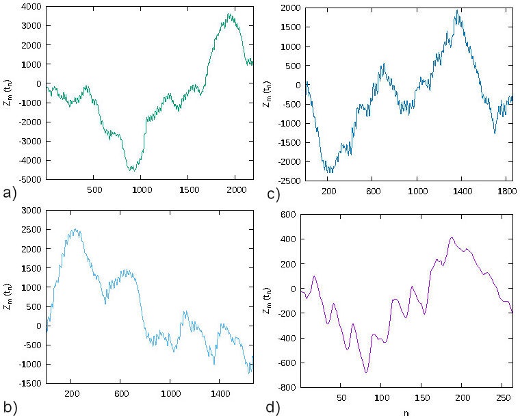
Figure 5 Fluctuation function associated with the O₃ c concentration variations corresponding to the year 2010 for: a) Spring, b) Summer, c) Autumn and d) Winter. 

Xm(tn) is obtained from x(t) for each season, where m = Spring, Summer, Autumn and Winter, tn∈[1,N] and n=1,2,3,4,… Note that Fig. 3 shows the variation of O₃ concentration profiles for each season of the year 2010 for CUA monitoring station, defined by xm(tn). It is also noted that the number of records varies according to the season and time of year considered. Using Eq. (1) in Xm(tn) gives the fluctuation function Zm(tn)=ym(tn)-y^(tn) where the cumulative sum is ym(tn)=∑‍Xm(tn). The hourly mean of the O₃ concentration variations can be seen in Fig. 4.

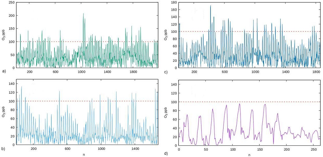
Figure 3 O₃ concentration variation of seasonal sites for CUA monitoring station in 2010: a) Spring, b) Summer, c) Autumn and d) Winter. 

Figure 4 O₃ concentration variations hourly mean in the 2010-2018 period for: a) MER, b) XAL, c) TLA and d) CUA. 

4 Analysis and discussion of results

4.1 Descriptive analysis

According to Fig. 2, the O₃ variation in four different monitoring stations (CUA, MER, TLA, and XAL) from January 1, 2010 to December 31, 2018, indicate the maximum levels allowed by the World Health Organization ^[45] and the Official Mexican Standard NOM-020-SSA1-2014 ^[46] for air quality. Note that the values above the dotted line indicate afflictions mainly in the airways and consequently the health of people. However, the O₃ concentration records that exceed the permissible threshold of 100 ppb have few incidents. The high occurrences index of maximum permissible O₃ observed throughout the study period suggests conducting studies in a contamination range of O₃ >100 ppb to neglect the existence of trends and was possibly due to situations that were atypical (see Table II).

Table II Number of occasions that concentration values were over 100 ppb, total in each station for the 2010-2018 period and total per season. 

Monitoring station	Spring	Summer	Autumn	Winter	2010-2018
MER	717	123	107	25	972
XAL	332	18	70	3	423
TLA	480	71	96	6	653
CUA	734	346	229	11	1320
Total	2263	558	502	45	3368

Meraz et al., observed a decrease in O₃ concentration in the nineties and non-decreasing seasonality for 2007, therefore it is stated that the dynamics of O₃ have changed dramatically in this studied decade ^[20].

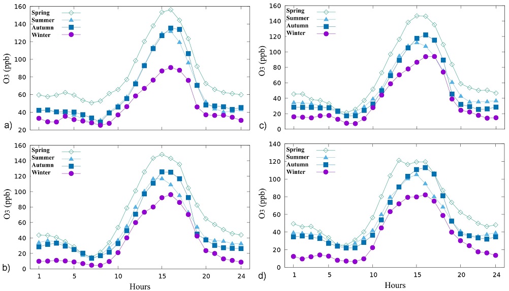
Figure 4 shows the O₃ record values for the different monitoring sites corresponding to: a) MER, b) XAL, c) TLA and d) CUA, for the analysis period 2010-2018. For each hour of the day, the values of O₃ records were averaged considering the data corresponding to each of the seasons of the year (spring, summer, autumn and winter), but not only for a single year, but for the entire period 2010-2018. It is observed that the maximum O₃ records occur in the range from 14 to 17 hrs with values ranging from 80 ppb to 160 ppb for the four sites and stations studied; analogous observations can be seen in ^[47-50]. We also note in this Fig. 4 that the magnitudes of the spring maximum O₃ records are always higher than the magnitudes of the winter maximum O₃ records. A similar behavior in O₃ concentration variations is maintained in different monitoring sites in Seul Corea for the four seasons of the year as observed by ^[51]. For the summer and fall at the four monitoring sites studied, the magnitude of the maximum records is lower than those observed in spring, but higher than those observed in winter. Locally, monitoring sites show diferences regard O₃ concentration levels. Higher values are found for MER, XAL, and TLA sites, while the lowest concentration values are observed for CUA.

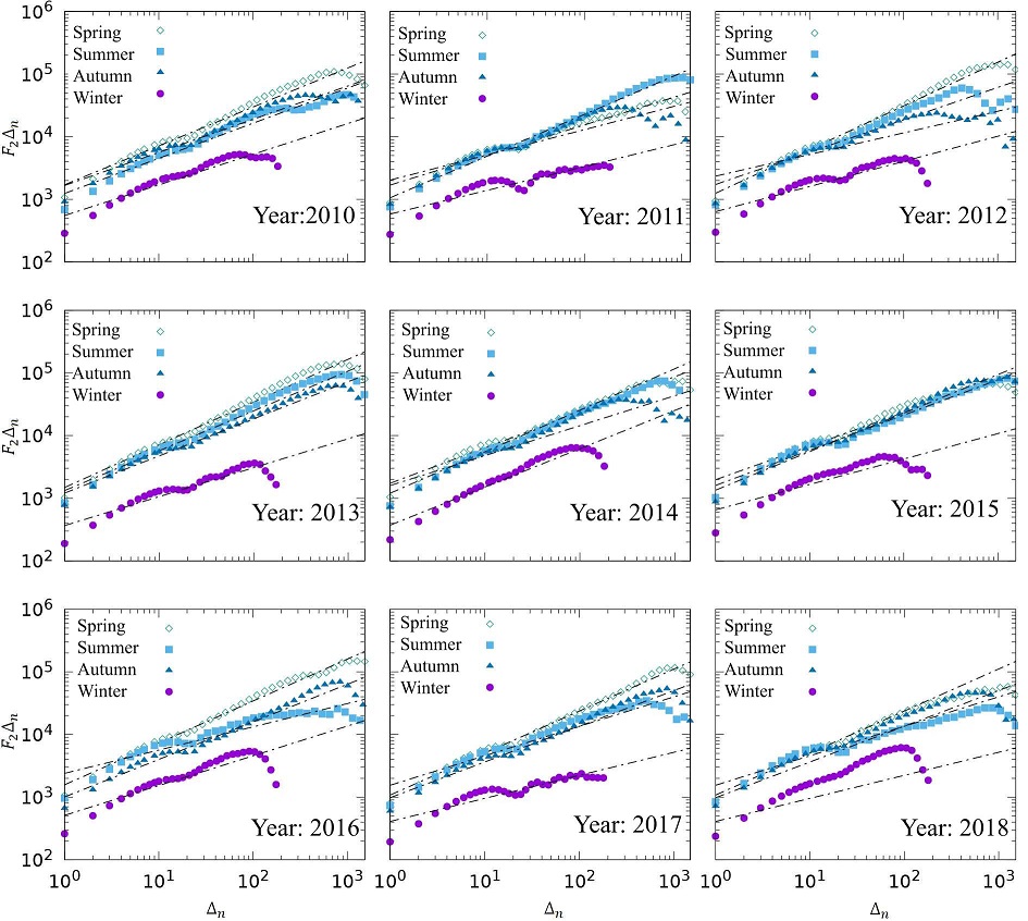
In addition, the maximum record values of the pollutant O₃, which exceed the limits allowed by the Mexican official standard NOM-020-SSA1-2021 and have led to environmental contingencies, are observed too in the spring, summer and winter seasons. Figure 5 shows the fluctuation function constructed from O₃ concentration profiles (Fig. 3) concentration variations of CUA for Spring, Summer, Autumn and Winter during 2010.

For the Structure function considering Spring, Summer, Autumn and Winter seasons corresponding to CUA, scaling in power law are consider to exist, according to the log-log graph of Fig. 6. It can be seen that the slope corresponds to H sampled from the four monitoring stations during the 2010-2018 period. An average value of H is estimated during the indicated period of the four monitoring zones for the Spring, Summer, Autumn and Winter seasons.

Figure 6 Structure function F2(Δn) for different Δn sizes for: Spring, Summer, Autumn and Winter from to CUA monitoring station. 

4.2 Structure function analysis

Figure 6 shows the scaling in power law of the fluctuations associated with O₃ concentration variation of the CUA monitoring station for the 2010-2018 period. Note that for Spring, Summer and Autumn seasons, it is observed a scale up to three orders of magnitude, where H is determined by the relation logF2(Δn)∼log(Δn)H. Table III, and Fig. 7 show the influence of temporality in the four monitoring stations. According, it is observed that the Spring season of the CUA, XAL, TLA, and MER monitoring stations predominates the trend of H to statistical persistence, with an occurrence rate of 63.8% and H¯=0.61, which implies that the O₃ concentration variation values subsequently registered and in process maintain the sign of the variations ^[32].

Table III H obtained in period 2010-2018 for each monitoring station. 

Season	Monitoring station	(H) Hurst exponent									Antipersistent	Randomness	Persistent
		2010	2011	2012	2013	2014	2015	2016	2017	2018
	MER	0.524	0.504	0.614	0.608	0.515	0.472	0.622	0.607	0.467
	XAL	0.434	0.668	0.620	0.627	0.428	0.424	0.575	0.533	0.588	0.45¯	0.50¯	0.61¯
	TLA	0.536	0.493	0.580	0.594	0.463	0.462	0.639	0.550	0.445	19.44%	16.67%	63.89%
	CUA	0.621	0.480	0.697	0.682	0.567	0.536	0.668	0.671	0.553
Summer	MER	0.512	0.636	0.478	0.520	0.528	0.449	0.419	0.487	0.311
	XAL	0.568	0.636	0.444	0.576	0.552	0.475	0.344	0.465	0.292	40¯	0.50¯	0.61¯
	TLA	0.487	0.637	0.414	0.585	0.536	0.452	0.519	0.491	0.438	33.33%	30.56%	36.11%
	CUA	0.560	0.666	0.516	0.636	0.626	0.562	0.371	0.471	0.391
Autumn	MER	0.535	0.358	0.424	0.519	0.407	0.55	0.499	0.521	0.429
	XAL	0.587	0.394	0.345	0.519	0.728	0.536	0.544	0.631	0.430	0.39¯	0.50¯	0.60¯
	TLA	0.583	0.313	0.442	0.516	0.334	0.554	0.508	0.549	0.414	36.11%	25%	38.89%
	CUA	0.529	0.403	0.345	0.59	0.478	0.615	0.599	0.571	0.512
Winter	MER	0.331	0.333	0.314	0.326	0.514	0.339	0.316	0.148	0.306
	XAL	0.475	0.168	0.289	0.319	0.396	0.297	0.373	0.160	0.368	0.32¯	0.50¯	0.58¯
	TLA	0.397	0.236	0.310	0.289	0.490	0.399	0.335	0.197	0.404	80.56%	16.67%	2.78%
	CUA	0.489	0.379	0.401	0.462	0.611	0.406	0.475	0.368	0.530

Figure 7 Hurst exponent distribution for year: a) Spring, b) Summer, c) Autumn and d) Winter. 

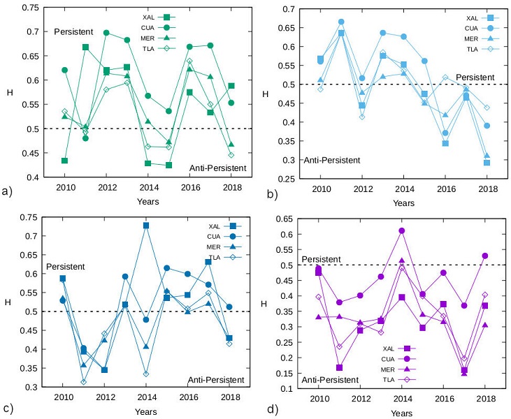
If the registered O₃ levels reach relatively high values, then the system tends to keep them high, indicating that it is limited by the scaling range where the power law predominates, and, consequently, the high O₃ values decrease to oscillate around a relatively low value, where the tendency is to maintain those values, until a transition occurs again. The trends of Hurts exponents seem to correspond to the climatic conditions of Mexico City, where, in Spring, a climatic variable in this season is the high heat condition due to increased solar radiation. Which would imply higher levels of O₃ concentration at this time, by its very nature of formation and, which corresponds to the time where O₃ concentration rates are high, as observed by ^[11,35]. For the Summer and Autumn seasons in the same monitoring stations, H reveals the three regimes with similar proportion of occurrence, summer 33.33%, which is antipersistent, followed by randomness with 30.56% and for persistence a rate of 36.11%. While for autumn there is an increase in the percentage of antipersistence with respect to summer of 36.11%, followed by a decrease with respect to the random regime with a percentage of 25%.

Finally, statistical persistence is characterized with a rate of 38.89%. In addition, Summer is an intermittence between hot days and rainy days, with greater and lesser solar radiation. This suggests high and low levels of O₃ concentration as reported by (Baldasano and Massagu_e 2017) where they found that pollutant records are lower during rainy times. In Autumn, the winds that help dissipate the O₃ predominate as reported by ^[52]. For Winter, the four monitoring stations show a well-defined Hurst exponent as antipersistent with an occurrence of 80.56%. This process indicates that the increments are independent and considered to be short memory processes.

The antipersistence in winter indicates that high or low O₃ concentration levels do not necessarily influence the values of subsequent records.

In Winter, the decrease in solar radiation predominates, which would indicate lower concentration levels as reported by ^[7]. In addition, the O₃ concentration records in this season can be mostly attributed to those caused by vehicular traffic. That is indicated by the high proportion of toluene and xylenes, found in hydrocarbons, as the main source as referred by ^[12]. Although this is a case study, the results suggest that could be associate persistence with warm seasons, i.e. with higher solar incidence and higher incidence of records with high O₃ concentration indices. While antipersistence, could be associate it with cold seasons, i.e., with lower solar incidence and lower incidence of high O₃ concentration records.

5 Conclusions

In this work it has been established that O₃ concentration levels are influenced by seasonal meteorological factors. The maximum values of O₃ concentration for a given hour of the day were observed during spring, while the minimum values were observed for winter. Between the two previous extremes were located the values for summer and autumn, which are very similar. This behavior is maintained throughout the study period, and it is independent of the monitoring site. Moreover, this behavior is congruent with the number of vehicle restriction measures taken by the city’s environmental authorities, which occur mostly in spring, summer and autumn. Locally, the monitoring sites do show differences in the magnitudes of O₃ concentrations; however, since the highest values correspond both to the most industrialized areas and to the areas with the highest vehicular traffic, this behavior can be associated to the anthropogenic activities of each monitoring site. It has been observed that the use of the fluctuation analysis and structure function technique are appropriate methods to characterize the power-law behavior (up to three orders of magnitude) of O₃ concentration levels for Mexico City. It was possible to characterize the power law trend of the O₃ fluctuation vs. time for each of the series of records for each season of the year by estimating the Hurst exponent. Using this method, it was possible to establish a correlation of persistence and antipersistence for spring and winter, respectively, in most cases. However, in some cases, the O₃ records show no correlation for the fluctuation function; that is, their processes are random. The Hurst exponent values for spring indicate statistical persistence and are therefore associated with long-range correlations. While those found for winter indicate statistical antipersistence, so they are associated with short-range correlations. On the other hand, the Hurst exponent values for summer and autumn were found to exhibit the three regimes of persistence, antipersistence and randomness, approximately in equal parts. Although this is a case study, the results suggest that could be associate persistence with warm seasons, i.e. with higher solar incidence and higher incidence of records with high O₃ concentration indices. While antipersistence, could be associate it with cold seasons, i.e., with lower solar incidence and lower incidence of high O₃ concentration records. Finally, due to the large number of incidences, higher than the maximum allowed levels of O₃ concentration in spring and summer, it is recommended that for a better understanding of the temporal and spatial evolution of O₃, a local analysis by zones and times of the year be considered; in addition to considering the influence of each of the anthropogenic variables specific to Mexico City.