1 Introduction

The photorefractive effect can be simply defined to be refractive index change as a function of incident intensity. An inhomogeneous light distribution excites charge carriers from donors and creates a charge concentration gradient. Charge transport through diffusion and/or drift and subsequent recombination at acceptor levels leads to a space charge field. The space charge electric field induces a refractive index change through the electro-optic effect. Self trapping or formation of spatial solitons can be realized in such photorefractives due to this index waveguide which leads to counteraction of diffraction. Hence, it is actually a robust balance between the nonlinearity and diffraction which leads to soliton formation in such materials.

Optical spatial solitons in photorefractive materials, which were theoretically predicted to exist in steady state ^[1,2] and demonstrated experimentally ^[3,4] have been an attractive topic for research ever since spanning a diverse range of investigations of the soliton characteristics ^[5-26]. The photorefractive effect can be said to correspond to a saturable nonlinearity and hence avoids the catastrophic collapse associated with the Kerr nonlinearity for 2+1 D solitons ^[27]. In addition, solitons are realizable in photorefractive media at relatively low laser powers(a few mW) and hence very convenient to observe experimentally. Potential practical applications of photorefractive solitons lie in the fields of optical switching, optical navigation, waveguiding, beam steering, optical computing, optical interconnects etc. ^[28-31].

There is a rich diversity of photorefractive solitons depending upon the type of nonlinearity in the photorefractive crystal (linear or quadratic or both) and the charge transport mechanism incorporating the drift and diffusion of charge carriers subsequently resulting in the formation of the space charge field. Screening solitons ^[1,32], photovoltaic solitons ^[33-35], screening photovoltaic solitons ^[21,36], pyroelectric solitons ^[20], screening photovoltaic pyroelectric solitons ^[37], centrosymmetric solitons ^[23], solitons in photorefractives having both linear and quadratic nonlinearity ^[38], photorefractive polymeric solitons ^[39,40] are some of the types of spatial solitons investigated in photorefractive materials.

The mechanism of the above mentioned solitons is the single photon photorefractive effect. Optical spatial solitons can be supported by the two-photon photorefractive effect also. The well-known model of Castro-Camus et al. ^[41] can be used to understand the two-photon photorefractive effect lucidly. According to this model, an intermediate level (IL) must be considered in addition to the valence band (VB) and conduction band (CB). A gating beam is assumed to provide a constant supply of excited electrons from the valence band subsequently excited to the conduction band by the signal beam. The signal beam induces a charge redistribution which then creates a space charge field. The space charge field results in an index waveguide through the electro-optic effect as before. Spatial soliton formation in such two-photon photorefractive media has been investigated in detail in previous researches ^[22,42-44].

An interesting mechanism which supports the self trapping process in photorefractives is the creation of a channel waveguide. The self defocusing of an optical beam induced by diffraction can be countered by the waveguiding effect and hence the waveguide supports the formation of solitons ^[12,19,45]. This results in lowering of the threshold power required to self trap a light beam as compared to the threshold power required in bulk photorefractive media. Photorefractive waveguides have attracted much interest recently with investigations of formation and propagation characteristics of solitons in waveguides embedded in different types of photorefractive crystals ^[12,19,45]. To the best of our knowledge, no one has investigated the self trapping in a photovoltaic photorefractive waveguide having two-photon photorefractive effect as yet and that will be our objective in this paper. We formulate the theory governing the existence and study the dynamical characteristics of the solitons in Secs. 2 and 3. In Sec. 4, we have investigate the stability of the solitons in the photorefractive waveguide by Lyapunov theory and numerical methods. Section 5 contains a brief summary of our results.

2 Theoretical foundation

Consider a light beam propagating in the z direction in a waveguide embedded in a photovoltaic photorefractive crystal. The optical c-axis of the photorefractive waveguide is coincident with the x-direction. The optical beam is polarized along the x-direction while we shall consider the diffraction to be along x-axis only. The electric field of the incident optical beam satisfies the following modified Helmholtz equation ^[12,19,45],

where k0 is the free space wave number and ne is the perturbed extraordinary index of refraction. can be found out from the expression of Δn in photorefractive materials ^[1],

where reff is the linear electro-optic coefficient and g is the waveguide parameter, usually taken as positive. This waveguide parameter represents in essence the strength of the index waveguide as can be seen clearly from (1). The electric field of the light beam is expressed as,

where Φ(x,z) denotes the slowly varying envelope of the wave and k=k0ne where k0 is the propagation constant in free space . We shall apply the paraxial approximation which implies that the z derivative of the amplitude function Φ(x,z) is a slowly varying function of z. Substituting (2) and (3) in (1) and making the paraxial approximation, we obtain,

E→sc=x^Esc is the space charge field setup in the photorefractive waveguide.

The expression for the space charge field in two photon photorefractive photovoltaic media neglecting the effect of diffusion can be stated ^[24],

where EP=KγNA/eμ is the photovoltaic field, Id=β/s2 is the dark irradiance, k is the photovoltaic constant, NA is the acceptor or trap density, γ is the recombination factor of the conduction to valence band transition, γ1 is the recombination factor for intermediate allowed level to valence band transition, β1 is the thermo ionization probability constant for transition from valence band to intermediate level. β2 is the thermo ionization probability constant for transition from intermediate level to conduction band. s1 and s2 are the photo ionization cross sections. I1 is the intensity of the gating beam which is constant. I2 refers to the beam intensity profile I∞ is the intensity at distances far from the centre, at x→±∞. Id is the contribution of thermal effects and hence called as dark irradiance while E0 refers to the value of the external electric field. In addition, the following dimensionless coordinates shall be adopted,

where x0 is an arbitrary spatial width which is used for scaling the transverse co-ordinate. Also, η=μ0/`o 0 Using these dimensionless coordinates, the evolution equation becomes,

Where

It is interesting to compare our dynamical evolution (6) with the corresponding equation for photovoltaic solitons in two-photon photorefractive crystals as derived in ^[24]. The authors in ^[24] investigate the photovoltaic solitons in photorefractive crystals without any embedded planar waveguide and hence the refractive index change is purely due to the electro-optic effect in the photorefractive crystal. We can see that the (13) of Ref. ^[24] is similar to our (6) but it does not contain the last term which signifies the strength of the waveguide. The effect of the embedded waveguide on the self trapping is the main aspect studied in this paper and hence the last term in (6) assumes significance.

Also, in (6), the non-linear variation of the refractive index results due to the fourth and fifth terms. By examining (6), we get to know that an exact analytical solution cannot be obtained. But there are several methods to approximately solve this equation. Segev’s method ^[32], Akhmanov’s paraxial method ^[46], Anderson’s variational method ^[47] and Vlasov’s moment method ^[48] can be used to solve (6). In our current analysis, we shall make use of the paraxial approximation and use a variational solution to obtain physically acceptable soliton states. Assume the slowly varying beam envelope to be of the form,

where A(ξ,s) is a purely real quantity and Ω(ξ,s) represents the phase. Substituting this ansatz in (6) and equating the real and imaginary parts to zero,

In (8), the first two terms represent the convergence or divergence of the beam and the third term represents the diffraction properties of the beam. The fourth, fifth and sixth terms elucidate the photovoltaic properties of the crystal. The fifth and sixth term in particular, represent the nonlinear terms contributing to the refractive index change. The last term in (8) is due to the planar waveguide structure in the photorefractive material. The last three terms control the diffraction effects and hence lead to a self trapped soliton propagation. The solution of (8) can be taken to be Gaussian. If we see ^[47], Anderson set a trend by suggesting the use of Gaussian profile in variational methods. Subsequently, this was implemented by many researchers in nonlinear optics ^{[12,19,49-58]}. Gaussian ansatz is most widely used for approximating solutions for non integrable systems and most widely used by the nonlinear optics and soliton community.

Firstly, Gaussian ansatz enables the calculations to become remarkably easier. Secondly, numerically computed exact profiles do not differ widely from the Gaussian one in most of the cases and thirdly, Gaussian profile is qualitatively very close to sech profile as it has almost the same half width and also the integral of the two profiles are comparable ^[47]. Finally, analytical simplification is not expected by using sech ansatz in most cases ^[58]. Since we use an approximate solution, we can term these solutions as quasi-solitons and henceforth the term soliton will refer to such quasi-solitons. We shall use the Gaussian ansatz of the form,

Here, P represents the normalized peak power of the soliton, r is a constant, a(ξ) represents the normalized beam width parameter and the product ra(ξ) gives us the spatial width of the soliton. The solution in (9) is taken to be a variational solution having a(ξ), Θ(ξ) and ψ(ξ) as the variational parameters which we need to obtain for physically acceptable soliton solutions. Ω(ξ,s) is basically the phase of the propagating soliton beam given as Ω(ξ,s)=12s2Θ(ξ)+ψ(ξ). The first term on the RHS, 12s2Θ(ξ)+ψ(ξ) signifies the phase in the transverse direction while the second term ψ(ξ) signifies the longitudinal phase.

In general, we can assume, a=1 at ξ=0 Also, it is quite logical to assume further that the soliton beam is not divergent at the entrance face of the photorefractive crystal and hence, da/dψ=0 at ξ=0.

Now, we know that ra(ξ) is the spatial width of the beam. If we have, a(ξ)=1 always, then we know that a stable propagating soliton forms of constant width r, hence we can also refer to r as equilibrium spatial width. After some algebraic simplification and retaining only first order terms, we obtain,

3 Existence of solitons

The above (10) illustrates the dynamical evolution of the beam width parameter and hence tells us about the variation of the spatial width itself. A self trapped beam results if the beam width remains constant. So we equate LHS of (10) to zero and obtain,

Equations (11) and (12) can be denoted to be an existence equation for bright solitons propagating stably through the photorefractive waveguide since it shows a relationship between the equilibrium spatial width (r), the threshold power (P0t) and the waveguide strength δ. The plot in Fig. 1 shows how this existence curve changes when we increase the strength of the waveguide δ. Equation (12) can be recast into a polynomial equation in terms of the threshold power P0t. The value of the threshold power may then be found out by solving the ensuing equation. This has been attempted and since the solution is a bit lengthy, it is shown in the Appendix. The parameters δ,η are positive and hence, we can see that bright solitons will be supported only in a material with a positive value of α. In the present analysis, we shall consider the following material parameters for illustration of our results ^{[21,22,41,59]}, ne=2.2, reff=30×10-12 m/V, s1=s2=3×10-4 m 2W -1s -1, β1=β2=0.05 s -1, γ1=3.3×10-17 m -3s -1, NA=1022 m -3, EP=4×106 V/m. Other parameters will be chosen as, I1=5×107 W/m 2, λ0=0.5×10-6 m, x0=10  μm. Based on these parameters, we get, α=22.19, η=3.33×10-6, α=6.6×10-6.

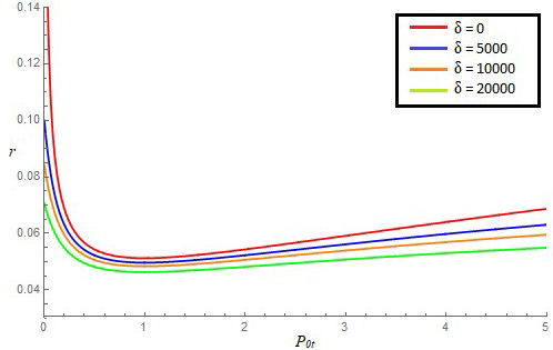
Figure 1 Existence curve in the presence of waveguiding showing the threshold power P0t as a function of equilibrium spatial width r when δ=0, 5000, 10000, 20000. 

Looking at the Fig. 1, we can infer the parameters of the solitons which can travel stably through the photorefractive waveguide. For stable soliton propagation, we can infer the threshold power P0t required for a particular soliton width very easily by seeing the existence curve shown in Fig. 1 considering the respective waveguide strength. We can see that the equilibrium spatial width r increases as the threshold power P0t tends towards zero. This implies that the spatial width of the soliton so formed increases with a decrease in the threshold power in the low power regime when P0t tends towards zero. The increase in the equilibrium spatial width of the soliton as P0t tends towards zero becomes more pronounced as the waveguiding strength becomes lesser. This is expected since the waveguide supports the self trapping of the soliton and a lesser value of the waveguide parameter will result in a weaker nonlinearity for self trapping and in turn a larger spatial width for the soliton.

Equation (12) has got four solutions or roots for the equilibrium spatial width parameter r. Inspection of the roots reveals that two roots are complex and hence they can be rejected as unphysical. Again, the third root is real but negative which can again be rejected as the soliton width cannot be negative. Hence, only one of the roots, which is positive and real can be identified to be the soliton width. From Fig. 1, we can infer that there are two values of the threshold power which are possible for a particular value of the equilibrium spatial width of the soliton. We can see that one of the values of the power lies in the low power regime and the other lies in the high power regime. This is the hallmark of bistable states. We shall identify the two threshold powers as P0t1 and P0t2. Bistability means the system has two stable equilibrium states and it can take either of the two values. Now, we define the two powers for which the soliton exists as “threshold powers” denoted by P0t1 and P0t2. The two “threshold” powers are simply denoting the two bistable states of the system.

We shall now try to understand the propagation behaviour of the solitons at different peak powers. We first consider the scenario in which there is no waveguiding effect and hence δ=0. Figure 2 shows the variation of the variable beam width parameter with distance of propagation. We have taken four distinct powers as follows, P1(=0.01)<P0t1, P2 (= 0.242) = P0t1, P0t1<P3(=2.5)<P0t2, P4(=25)>P0t2(=4.1). For clarity, we can take P5=P0t2(=4.1).

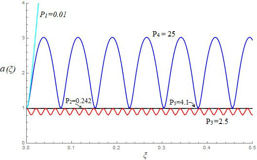
Figure 2 Soliton evolution shown by the variation in the beam width parameter a(ξ) with normalized distance for different peak powers. 

When the peak power is equal to P1, the beam width diverges to a large value because the light beam’s power is much less than the threshold power P0t1 required to self trap the beam. Hence, a stable soliton cannot form in such a case. Again, if the light beam’s power is exactly equal to the threshold power P0t1 or P0t2, we can see that the spatial width remains constant and hence results in stable self trapping. If the beam’s peak power lies between P0t1 or P0t2, we can see that the spatial width of the light beam oscillates but with an amplitude of oscillation less than unity. This can also be termed to be stable self trapping and the beam interpreted as a soliton. But when the peak power is greater than P0t2, we can see that the spatial width of the light beam oscillates with an amplitude of oscillation greater than 1 and hence self trapping cannot be said to take place in such a case. Figures 3 to 6 show the dynamical evolution of the soliton for these above mentioned cases respectively and reinforce the existence of four separate power regions.

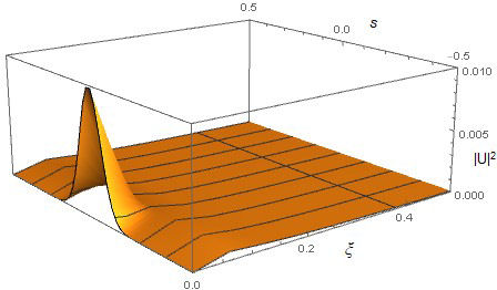
Figure 3 Dynamical evolution of the soliton beam in the absence of waveguiding( δ=0) with power less than the first threshold power, P1(=0.01)<P0t1. 

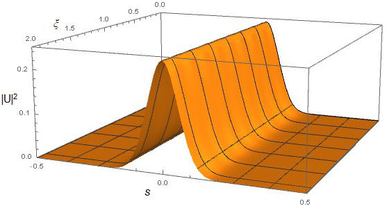
Figure 4 Dynamical evolution of the soliton beam in the absence of waveguiding( δ = 0) with power equal to the threshold power, P2(=0.242)=P0t1 or P5(=4.1). 

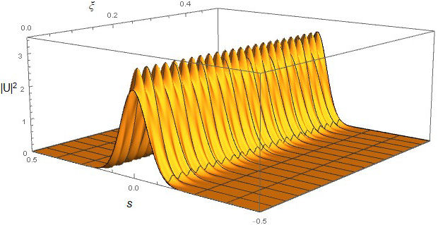
Figure 5 Dynamical evolution of the soliton beam in the absence of waveguiding ( δ=0) with power P=2.5, i.e., power lying between the two threshold powers P0t1 and P0t2. 

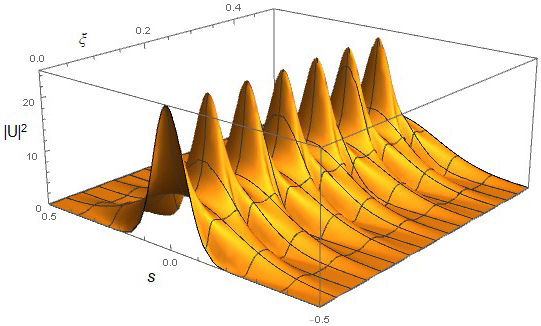
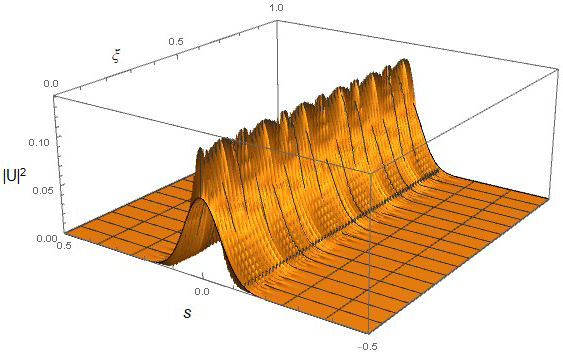
Figure 6 Dynamical evolution of the soliton beam in the absence of waveguiding ( δ=0) with power greater than the second threshold power, P4(=25)>P0t2(=4.1). 

In Fig. 3, we can see a stable soliton does not form and diverges because the power is less than the threshold power P0t1 needed to form the soliton. In Fig. 4, we see the formation of a perfect soliton since the power now equals the threshold power, either P0t1 or P0t2. In Fig. 5, since the power of the light beam lies between the two threshold powers P0t1 and P0t2, we can see a sort of self trapping happening. As mentioned before, even though the spatial width and amplitude are oscillating, the oscillation amplitude is less than unity and this can be termed as a soliton. But in Fig. 6, when the light beam’s power is increased to greater than P0t2, we can clearly infer that the travelling light beam is not a soliton since its spatial width and amplitude oscillate with an amplitude greater than unity.

Next, we shall investigate the effect of the waveguide on the propagation of the light beam within the photorefractive crystal. Solving (11) for different values of δ, we have plotted the soliton’s evolution while propagating. We have chosen the value of power P and r such that P is less than the threshold power P0t1 for that particular value or r. We take r=0.0808 and we have chosen the beam’s peak power P=0.08. From the existence curve in Fig. 1, we infer that the power P=0.08 is less than the threshold power needed to form a soliton for the particular r=0.0808. Since the peak power is less than the threshold power, we expect no self trapping or self focussing in absence of any other intervention and hence it is interesting wish to see the influence of the waveguide on the propagation characteristics of such a light beam.

Figure 7 graphically shows how the beam width changes with propagation distance. For the unguided case, i.e., δ=0, we can see that the light beam’s spatial profile diverges sharply and hence self trapping does not take place. As we increase the strength of the waveguide (by increasing δ), we can clearly see some sort of self trapping effect. At a particular value of the waveguide strength ( δ=6500), the beam width equals one and remains constant with propagation. Hence, a perfectly self trapped beam, i.e., soliton can be clearly inferred to exist here. The waveguide enhances the nonlinearity induced self focussing and is just enough to enable the formation of a perfectly self trapped beam or soliton of width ra(ξ)=0.0808. As we keep on increasing the waveguide parameter to above this particular value, the beam width starts to oscillate with propagation but the amplitude of oscillation is less than unity. Such beams can also be said to be self trapped and hence referred to as solitons. The important observation here is that a soliton could be realized even at peak power less than the threshold power in such two photon photovoltaic photorefractive material due to the self focussing provided by the planar waveguide. The higher we choose the waveguide parameter, the lower will be our required peak power to realize a soliton within the crystal. Figure 8-12 show the aforementioned cases by plotting the soliton’s dynamical evolution with distance explicitly. In Fig. 8, we can see that the soliton diverges as the waveguide strength is zero and the power of the soliton is less than the threshold power required for self trapping. As we increase the waveguide strength by increasing the waveguide parameter, we can see some sort of self trapping in Fig. 9, but it cannot be called as a soliton beam since the beam width oscillates with propagation and the amplitude of oscillation is greater than unity. As we increase the waveguide parameter further, for δ=6500, we can see the propagation of a perfect soliton in Fig. 10. For further increases in the waveguide parameter, in Figs. 11 and 12, we can see some sort of self trapping and hence these can also be called solitons since the beam width oscillates with propagation but the amplitude of oscillation is less than unity.

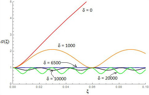
Figure 7 Soliton evolution shown by the variation in the beam width parameter a(ξ) with normalized distance for different waveguide strengths. P=0.08, r=0.0808. 

Figure 8 Dynamical evolution of the soliton beam ( δ=0), P=0.08, r=0.0808. 

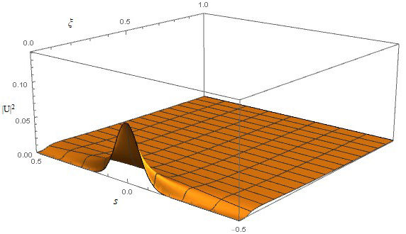
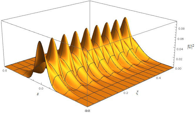
Figure 9 Dynamical evolution of the soliton beam in the presence of waveguiding ( δ=1000), P=0.08, r=0.0808. 

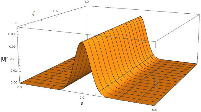
Figure 10 Dynamical evolution of the soliton beam in the presence of waveguiding ( δ=6500), P=0.08, r=0.0808. 

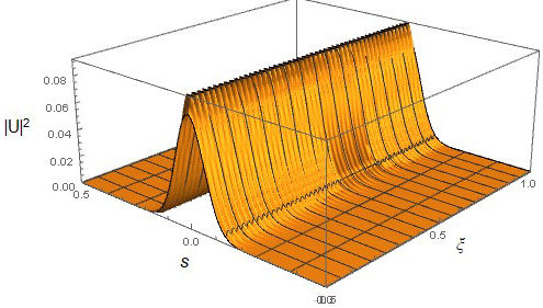
Figure 11 Dynamical evolution of the soliton beam in the presence of waveguiding ( δ=10000), P=0.08, r=0.0808. 

Figure 12 Dynamical evolution of the soliton beam in the presence of waveguiding ( δ=20000), P=0.08, r=0.0808. 

4 Linear stability analysis

At this point, it is important that we investigate the stability of the solitons propagating inside the photorefractive waveguide since only stable solitons have potential practical applications. It will be in order to revisit the Eq. (11) and define new quantities ζ, F, X such that,

And

In Eq. (13), as a general case, da/dξ has been defined to be a new function F(a,ζ) and in particular, F(a,ζ)=ζ. F is a function while ζ is a variable. Similar arguments can be used to understand the function in Eq. (14). Equation (14) has been obtained by using Eqs. (11) and (13). Equations (13) and (14) now serve as the point for starting our investigation into the stability of solitons using Lyapunov’s exponent ^[60]. Since we consider the linear stability, we shall write the variables to consist of a steady state value and a very small perturbation term. So, a=as+a^ and ζ=ζs+ζ^ where the subscript s represents the steady state values and a^ and ζ^ represent the small perturbations in a and ζ respectively. Substituting in (13) and (14) and linearizing the ensuing expression, we get,

where,

and

Constructing a Jacobian determinant and equating to zero for a non trivial solution,

Solving (17), we get,

where,

and

Following Lyapunov, we can conclude that steady state solutions of (13)-(14) will be stable if λ is not positive. The two eigenvalues of the above equation (19) come out to be

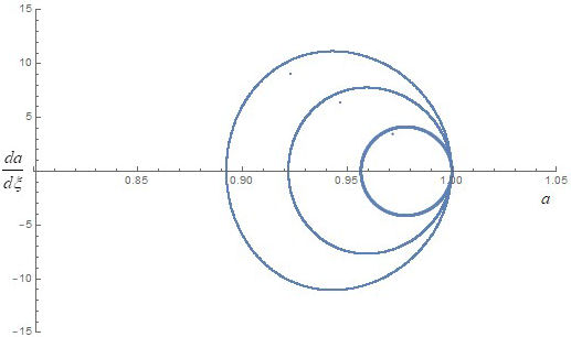
Since both the roots come out to be imaginary, we can conclude that the solitons are stable. This can be verified numerically also by investigating the behaviour of solitons in the phase plane under small perturbations. The variation in spatial width a is plotted in Figs. 13-15 under small perturbations. The perturbation ranges from 5% to 15%. The stability of solitons is inferred by the closed trajectories.

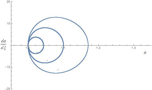
Figure 13 Phase trajectory of the spatial soliton resulting from the perturbation in its value at steady state. The perturbation ranges from 5% to 15% and a low power regime has been considered. ( P≪1) (perturbed power less than P0t1). 

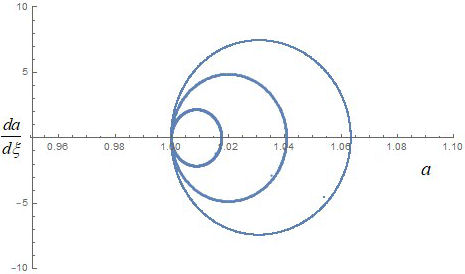
Figure 14 Phase trajectory of the spatial soliton resulting from the perturbation in its value at steady state. The perturbation ranges from 5% to 15% and a high power regime has been considered. (P≫1) (perturbed power greater than P0t1). 

Figure 15 Phase trajectory of the spatial soliton resulting from the perturbation in its value at steady state. The perturbation ranges from 5% to 15% above P0t1 and hence the perturbed power lies between P0t1 and P0t2. 

5 Conclusion

We have investigated the existence, propagation and characteristics of optical spatial solitons in a waveguide embedded in a two photon photovoltaic photorefractive crystal. In the absence of waveguiding, we have identified four distinct regimes of power and investigated the dynamical evolution of the solitons in all of these. We also observe the presence of bistable states. We then study the effect of the waveguide parameter or the strength of the waveguide on the self trapping. The planar waveguide enhances the self focussing due to the photorefractive nonlinearity resulting in lessening of the threshold power required to support steady state self trapping. The higher is the considered value of the waveguide parameter or the waveguoide strength, the lower is the threshold power required to self trap a soliton. Finally, we have investigated the linear stability of such solitons analytically and also by numerical simulations which reveal that they are stable against small perturbations.

Data availability statement

The data that support the findings of this study are available from the author, upon reasonable request.

References

1. D. N. Christodoulides and M. I. Carvalho, Bright, dark, and gray spatial soliton states in photorefractive media J. Opt. Soc. Am. B 12 (1995) 1628 https://dx.doi.org/10.1364/JOSAB.12.001628. [ Links ]
2. M. Segev, G. C. Valley, B. Crosignani, P. Diporto, and A. Yariv, Steady-state spatial screening solitons in photorefractive materials with external applied field Phys. Rev. Lett. 73 (1994) 3211. https://doi.org/10.1103/PhysRevLett.73.3211. [ Links ]
3. Z. Chen, M. H. Garrett, G. C. Valley, M. Mitchell, M. Shih, and M. Segev, Steady-state dark photorefractive screening solitons Opt. Lett. 21 (1996) 629, https://dx.doi.org/10.1364/OL.21.000629. [ Links ]
4. K. Kos, H. Meng, G. Salamo, M. M. Shih, M. Segev, and G. C. Valley, One-dimensional steady-state photorefractive screening solitons, Phys Rev E Stat Phys Plasmas Fluids Relat Interdiscip Top. 53 (1996) R4330 https://dx.doi.org/10.1103/PhysRevE.53.R4330. [ Links ]
5. M. Segev, B. Crosignani, A. Yariv, Self-trapping of optical beams in photorefractive media, Front. Nonlinear Opt. Sergei Akhmanov Memorial Volume, (CRC Press, Boca Raton, 2021) pp. 136. [ Links ]
6. Q. Jiang, Y. Su, Z. Ma, and J. Chen, Coherent interactions of multi-Airy-Gaussian beams in photorefractive media J. Opt., 49 (2020) 224. https://doi.org/10.1007/s12596-020-00610-w. [ Links ]
7. Q.-S. Liu, Z.-X. Zhang, H. Cui, Z.-C. Luo, W.-C. Xu, and A.-P. Luo, Generation and manipulation of spiral beams in photovoltaic photorefractive crystal twinning with mirroring diffusion management Opt. Commun., 478 (2021) 126331 https://doi.org/10.1016/j.optcom.2020.126331. [ Links ]
8. A. Katti, Coupling of separate solitons in a series circuit of two photon photorefractive crystals exhibiting simultaneous quadratic and linear nonlinearities Optik, 206 (2020) 164212 https://doi.org/10.1016/j.ijleo.2020.164212. [ Links ]
9. G. Di Domenico, Introduction to Nonlinear Optics in Photorefractive Media, Electro-optic Photonic Circuits, (Springer, Switzerland, 2019) pp. 1-17. https://doi.org/10.1007/978-3-030-23189-7_1. [ Links ]
10. Q. Jiang, Y. Su, H. Nie, Z. Ma, and Y. Li, Propagation and interaction of finite-energy Airy-Hermite-Gaussian beams in photorefractive media Appl. Phys. B, 124 (2018) 1. https://doi.org/10.1007/s00340-018-6906-0. [ Links ]
11. X. Zhang, G. Zhang, and H. Zhou, The evolution and deflection characteristics of Gaussian beam in photovoltaic photorefractive crystal circuit with dark soliton intensity effect Optik, 160 (2018) 182. https://doi.org/10.1016/j.ijleo.2018.01.097. [ Links ]
12. B. P. Akhouri and P. K. Gupta, Waveguiding effect on optical spatial solitons in centrosymmetric photorefractive materials J. Opt., 46 (2017) 281 https://dx.doi.org/10.1007/s12596-016-0372-z. [ Links ]
13. L. Hao, C. Hou, Q. Wang, and H. Mu, Coherently coupled spatial soliton pairs in biased photorefractive crystals with both the linear and quadratic electro-optic effects Optik, 127 (2016) 4339. https://doi.org/10.1016/j.ijleo.2016.01.143. [ Links ]
14. T. Zhao, T. Bo, J. Yan, W. Pan, and L. Min, Dynamics of the Manakov solitons in biased guest-host photorefractive polymer Commun. Theor. Phys. 60 (2013) 150 https://doi.org/10.1088/0253-6102/60/2/02. [ Links ]
15. X. Ji, Q. Jiang, and J. Liu, Separate spatial holographic and two-photon-Hamiltonian soliton pairs in an unbiased series photorefractive crystal circuit Optik, 123 (2012) 1223 https://dx.doi.org/10.1016/j.ijleo.2011.07.055. [ Links ]
16. L. Keqing, T. Tiantong, and Z. Yanpeng, One-dimensional steady-state spatial solitons in photovoltaic photorefractive materials with an external applied field Phys. Rev. A, 61 (2000) 053822 https://dx.doi.org/10.1103/PhysRevA.61.053822. [ Links ]
17. L. Keqing, Z. Yanpeng, T. Tiantong, and L. Bo, Incoherently coupled steady-state soliton pairs in biased photorefractive-photovoltaic materials Phys. Rev. E-Stat. Nonlinear Soft Matter Phys. 64 (2001) 056603 https://dx.doi.org/10.1103/PhysRevE.64.056603. [ Links ]
18. C. F. Hou and L. Wang, Manakov solitons in biased photorefractive polymer Optik 115 (2004) 405 https://dx.doi.org/10.1078/0030-4026-00389. [ Links ]
19. A. Katti, Bright pyroelectric quasi-solitons in a photorefractive waveguide Optik, 156 (2018) 433, https://dx.doi.org/10.1016/j.ijleo.2017.10.105. [ Links ]
20. J. Safioui, F. Devaux, and M. Chauvet, Pyroliton: pyroelectric spatial soliton. Opt. Express, 17 (2009) 22209 https://dx.doi.org/10.1364/OE.17.022209. [ Links ]
21. J. S. Liu and K. Q. Lu, Screening-photovoltaic spatial solitons in biased photovoltaic-photorefractive crystals and their self-deflection J. Opt. Soc. Am. B -Opt. Phys., 16 (1999) 550 https://doi.org/10.1364/JOSAB.16.000550. [ Links ]
22. C. Hou, Y. Pei, Z. Zhou, and X. Sun, Spatial solitons in two-photon photorefractive media Phys. Rev. A , 71 (2015) 053817 https://doi.org/10.1103/PhysRevA.71.053817. [ Links ]
23. M. Segev and A. J. Agranat, Spatial solitons in centrosymmetric photorefractive media Opt. Lett. 22 (1997) pp. 1299 https://dx.doi.org/10.1364/OL.22.001299. [ Links ]
24. C. Hou, Y. Zhang, Y. Jiang, and Y. Pei, Photovoltaic solitons in two-photon photorefractive materials under open-circuit conditions Opt. Commun. 273 (2007) 544 https://dx.doi.org/10.1016/j.optcom.2007.01.024. [ Links ]
25. B. Hanna et al., Spatial solitons in photorefractive lattices Optoelectron. Rev. 13 (2005) 85. [ Links ]
26. B. Kumari, P. M. Z. Hasan, R. Darwesh, P. A. Alvi, and A. Katti, Separate coupled solitons in biased series photorefractive semiconductor circuit Laser Phys. 31 (2021) 085401 https://doi.org/10.1088/1555-6611/ac089c. [ Links ]
27. M. Segev, Optical spatial solitons Opt. Quantum Electron. 30 (1998) 503. https://doi.org/10.1023/A:1006915021865. [ Links ]
28. Z. Chen, M. Segev , and D. N. Christodoulides, Optical spatial solitons: historical overview and recent advances Rep. Prog. Phys. 75 (2012) 086401 https://dx.doi.org/10.1088/0034-4885/75/8/086401. [ Links ]
29. S. Trillo and W. E. Torruellas, Eds., Spatial Solitons, Springer Series in Optical Sciences, vol. 31. (Springer, Berlin, 2001.) [ Links ]
30. G. I. Stegeman, Optical Spatial Solitons and Their Interactions: Universality and Diversity Science, 286 (1999) 1518 https://dx.doi.org/10.1126/science.286.5444.1518. [ Links ]
31. D. D. Nolte, Photorefractive Effects and Materials. (Springer Science & Business Media, New York, 2013). [ Links ]
32. M. Segev , B. Crosignani, A. Yariv, and B. Fischer, Spatial solitons in photorefractive media Phys. Rev. Lett. , 68 (1992) 923, https://dx.doi.org/10.1103/PhysRevLett.68.923. [ Links ]
33. G. C. Valley, M. Segev , B. Crosignani, A. Yariv, M. M. Fejer, and M. C. Bashaw, Dark and bright photovoltaic spatial solitons Phys. Rev. A , 50 (1994) R4457 https://dx.doi.org/10.1103/PhysRevA.50.R4457. [ Links ]
34. M. Segev , G. C. Valley, M. C. Bashaw, M. Taya, and M. M. Fejer, Photovoltaic spatial solitons J. Opt. Soc. Am. B , 14 (1997) 1772 https://dx.doi.org/10.1364/JOSAB.14.001772. [ Links ]
35. M. Taya, M. C. Bashaw, M. M. Fejer, M. Segev , and G. C. Valley, Observation of dark photovoltaic spatial solitons Phys. Rev. A , 52 (1995) 3095 https://doi.org/10.1103/PhysRevA.52.3095. [ Links ]
36. E. Fazio et al., Screening-photovoltaic bright solitons in lithium niobate and associated single-mode waveguides Appl. Phys. Lett. 85 (2004) 2193, https://doi.org/10.1063/1.1794854. [ Links ]
37. A. Katti and R. A. Yadav, Spatial solitons in biased photovoltaic photorefractive materials with the pyroelectric effect Phys. Lett. Sect. Gen. At. Solid State Phys. 381 (2017) 166 https://doi.org/10.1016/j.physleta.2016.10.054. [ Links ]
38. L. Hao, Q. Wang, and C. Hou, Spatial solitons in biased photorefractive materials with both the linear and quadratic electro-optic effects J. Mod. Opt., 61 (2014) 1236, https://dx.doi.org/10.1080/09500340.2014.928379. [ Links ]
39. M. F. Shih and F. W. Sheu, Photorefractive polymeric optical spatial solitons. Opt. Lett. , 24 (1999) 1853 https://dx.doi.org/10.1364/OL.24.001853. [ Links ]
40. F.-W. Sheu and M.-F. Shih, Photorefractive polymeric solitons supported by orientationally enhanced birefringent and electro-optic effects J. Opt. Soc. Am. B , 18 (2001) 785 https://dx.doi.org/10.1364/JOSAB.18.000785. [ Links ]
41. E. Castro-Camus and L. F. Magana, Prediction of the physical response for the two-photon photorefractive effect Opt. Lett. 28 (2003) 1129. https://doi.org/10.1364/OL.28.001129. [ Links ]
42. L. Hao, C. Hou, and Q. Wang, Spatial solitons in biased two-photon photorefractive crystals with both the linear and quadratic electro-optic effect Opt. Laser Technol. 56 (2014) 326 https://dx.doi.org/10.1016/j.optlastec.2013.09.013. [ Links ]
43. G. Zhang and J. Liu, Screening-photovoltaic spatial solitons in biased two-photon photovoltaic photorefractive crystals J. Opt. Soc. Am. B , 26 (2009) 113 https://doi.org/10.1364/JOSAB.26.000113. [ Links ]
44. K. Zhan, C. Hou, H. Tian, S. Pu, and Y. Du, Spatial solitons in centrosymmetric photorefractive crystals due to the two-photon photorefractive effect J. Opt. 12 (2010) 015203 https://doi.org/10.1088/2040-8978/12/1/015203. [ Links ]
45. A. Katti, R. A. Yadav, and A. Prasad, Bright optical spatial solitons in photorefractive waveguides having both the linear and quadratic electro-optic effect Wave Motion, 77 (2018) 64 https://doi.org/10.1016/J.WAVEMOTI.2017.10.002. [ Links ]
46. S. A. Akhmanov, A. P. Sukhorukov, and R. V. Khokhlov, Self-Focusing and Difraction of Light Beams in a Nonlinear Medium Sov. Phys. Uspekhi, 10 (1968) 609 https://doi.org/10.1070/PU1968v010n05ABEH005849. [ Links ]
47. D. Anderson, Variational approach to nonlinear pulse propagation in optical fibers Phys. Rev. A , 27 (1983) 3135 https://doi.org/10.1103/PhysRevA.27.3135. [ Links ]
48. S. N. Vlasov, V. A. Petrishchev, and V. I. Talanov, Averaged description of wave beams in linear and nonlinear media (the method of moments) Radiophys. Quantum Electron., 14 (1974) 1062 https://doi.org/10.1007/BF01029467. [ Links ]
49. B. Malomed, D. Anderson , M. Lisak, M. L. Quiroga-Teixeiro, and L. Stenflo, Dynamics of solitary waves in the Zakharov model equations Phys. Rev. E, 55 (1997) 962. https://doi.org/10.1103/PhysRevE.55.962. [ Links ]
50. V. Skarka, V. I. Berezhiani, and R. Miklaszewski, Spatiotemporal soliton propagation in saturating nonlinear optical media Phys. Rev. E - Stat. Phys. Plasmas Fluids Relat. Interdiscip. Top., 56 (1997) 1080 https://doi.org/10.1103/PhysRevE.56.1080. [ Links ]
51. V. Skarka and N. B. Aleksić, Stability criterion for dissipative soliton solutions of the one-, two-, and three-dimensional complex cubic-quintic Ginzburg-Landau equations Phys. Rev. Lett. 96 (2006) 013903. https://doi.org/10.1103/PhysRevLett.96.013903. [ Links ]
52. Z. Liu, W. Zang, J. Tian, W. Zhou, C. Zhang, and G. Zhang, Analysis of Z-scan of thick media with high-order nonlinearity by variational approach Opt. Commun. 219 (2003) 411 https://doi.org/10.1016/S0030-4018(03)01298-7. [ Links ]
53. Y. Huang, Q. Guo, and J. Cao, Optical beams in lossy non-local Kerr media Opt. Commun. 261 (2006) 175. https://doi.org/10.1016/j.optcom.2005.12.003. [ Links ]
54. S. Jana and S. Konar, A new family of Thirring type optical spatial solitons via electromagnetically induced transparency Phys. Lett. A 362 (2007) 435. https://doi.org/10.1016/j.physleta.2006.10.043. [ Links ]
55. P. T. Dinda, A. B. Moubissi, and K. Nakkeeran, A collective variable approach for dispersion-managed solitons J. Phys. Math. Gen. 34 (2001) L103. https://doi.org/10.1088/0305-4470/34/10/104. [ Links ]
56. J. Santhanam, C. J. McKinstrie, T. I. Lakoba, and G. P. Agrawal, Effects of precompensation and postcompensation on timing jitter in dispersion-managed systems Opt. Lett. , 26 (2001) 1131. https://doi.org/10.1364/OL.26.001131. [ Links ]
57. J. H. B. Nijhof, W. Forysiak, and N. J. Doran, The Averaging Method for Finding Exactly Periodic dispersion-managed solitons IEEE J. Sel. Top. Quantum Electron. 6 (2000) 330. https://doi.org/10.1109/2944.847768. [ Links ]
58. J. N. Kutz, S. D. Koehler, L. Leng, and K. Bergman, Analytic study of orthogonally polarized solitons interacting in highly birefringent optical fibers J. Opt. Soc. Am. B - Opt. Phys. 14 (1997) 636. https://doi.org/10.1364/JOSAB.14.000636. [ Links ]
59. B. Liu, L. Liu, and L. Xu, Characteristics of recording and thermal fixing in lithium niobate Appl. Opt. 37 (1998) 2170. https://doi.org/10.1364/AO.37.002170. [ Links ]
60. I. Prigogine, G. Nicolis, Self-Organisation in Nonequilibrium Systems: Towards A Dynamics of Complexity. In: Hazewinkel, M., Jurkovich, R., Paelinck, J.H.P. (eds) Bifurcation Analysis. (Springer, Dordrecht, 1985). [ Links ]
How to Cite. A. Katti, “Bright optical spatial solitons in a photovoltaic photorefractive waveguide exhibiting the two photon photorefractive effect”, Rev. Mex. Fís., vol. 69, no. 2 Mar-Apr, pp. 021301 1-, Mar. 2023.
Appendix A
We have, from (12),
1r4=1r22aηP0t+2aηδP0t(1+P0t)2+2δ. (A.1)
Simplifying, we get
(1+P0t)2=2αηr2P0t(1+P0t)2+2αηδr2P0t+2δr4(1+P0t)2. (A.2)
Equation (A.2) is a polynomial equation of order three which can be solved to get the threshold power P0t,
P0t=1-2r4δ-4r2αη6r2αη+(-(1-2r4δ-4r2αη)2+12r2αη(-1+2r4δ+r2αη+r2αηδ))3(22/3)r2αη-2+12r4δ-24r8δ2+16r12δ3-12r2αη+48r6αδη-48r10αδ2η-24r4α2η2+48r8α2δη2-16r6α3η3+36r4α2η2σ-72r8α2δη2σ-144r6α3η3σ+((-2+12r4δ-24r8δ2+16r12δ3-12r2αη+48r6αδη-48r10αδ2η-24r4α2η2+48r8α2δη2-16r6α3η3+36r4α2η2σ-72r8α2δη2σ-144r6α3η3σ)2+4(-(1-2r4δ-4r2αη)2)+12r2αη(-1+2r4δ+r2αησ))3)1/21/3-16(2)1/3r2αη-2+12r4δ-24r8δ2+16r12δ3-12r2αη+48r6αδη-48r10αδ2η-24r4α2η2+48r8α2δη2-16r6α3η3+36r4α2η2σ-144r6α3η3σ+((-2+12r4δ-24r8δ2+16r12δ3-12r2αη+48r6αδη-48r10αδη-24r4α2η2+48r6α2δη2-16r6α3η3+36r4α2η2σ-72r8α2δη2σ-144r6α3η3δ)2+4(-(1-2r4δ-4r2αη)2+12r2αη(-1+2r4δ+r2αη+r2αησ))3)1/21/3. (A.3)
Received: March 27, 2022; Accepted: June 21, 2022
Creative Commons License This is an open-access article distributed under the terms of the Creative Commons Attribution License