1. Introduction

Over the past few years, it has been demonstrated that a wide range of homogeneous and inhomogeneous phases, in equilibrium and nonequilibrium, in both simple and complex fluids, can be modulated simply by changing the range and strength of the interaction potential [¹-⁴]. This is due to the superposition of repulsive and attractive contributions in the interaction potential; i.e., the physical behavior of the observed phases results from the competition between different types of interactions, leading to complex potentials between fluid particles [⁵-¹¹, ¹³-²⁵]. Competing interactions have been widely used to investigate, for example, the formation of ordered structures in complex systems, such as globular protein solutions [⁵-⁷], the effective interactions between solute particles in a subcritical solvent [⁸], the temperature dependence of cluster-like formations in double-Yukawa fluids [⁹-¹²], and the microphase separations in two- and three-dimensional systems [¹³-²¹]. In particular, A. Santos et al. [²⁵] studied the structural properties of fluids whose molecules interact via potentials with a hard core plus two piece-wise constant sections of different widths and heights, using the rational-function approximation method. A similar fluid with a square well-barrier potential was studied with excellent results.

From the structural point of view, a macroscopic or thermodynamic phase separation in monodisperse fluids can be represented using the divergence of the static structure factor S(q) at q = 0 in the long wavelength limit [²⁶]. In contrast, a microphase separation refers to the presence of a peak in S(q) at wavelengths q ≤ q _m (≡2π/d), where d is either the particle diameter or the mean interparticle distance. Further details on the definition of microphase separation are provided by A. Archer and co-workers [¹⁶-²¹]. This characteristic peak is associated with a type of particle aggregation [⁵]. However, it is still debatable whether such a peak indicates a correlation between aggregates, i.e., clusters, in the fluid or represents an intermediate range order structure [²⁷]. Nonetheless, the degree of ordering of the aggregate should be a function of the peak height, although this parameter does not provide explicit information about the type of ordering and the possible transition from intermediate to permanent order. Further studies in this direction are discussed elsewhere [²⁸].

Hence, in this work, the term microphase separation is simply used to highlight the presence of an additional peak in S(q) at low-q values, which is driven by competition between attractive and repulsive contributions of interaction potential. Commonly, a continuous interaction potential that considers short-range attraction and long-range repulsion, i.e., a double-Yukawa potential, is used to represent a wide variety of systems with competing interactions [⁹-¹¹, ¹³-²¹]. Here we follow a different strategy and consider a potential represented by a superposition of square-wells and square-barriers. A fluid in which particles interact with this kind of potential is usually known as a discrete potential fluid (DPF) [²⁹]. DPFs are important since they allow to study separately the effects produced by the different attractive and repulsive components of the potential [³⁰, ³²]; an aspect that cannot be investigated using continuous potentials, where only global effects can be distinguished. The thermodynamic and structural properties of DPFs have been studied by computer simulations, perturbation-like theories, and integral equations theory [³², ³³, ³⁵-⁴²]. Furthermore, DPFs have been found to exhibit multiple phase transitions [³⁰, ³¹]. Analytical expressions for direct correlation functions have been developed [⁴³-⁴⁶], which could be used as new reference systems in perturbation-like theories or incorporated into dynamical approaches [⁴⁷, ⁴⁸] considering the diffusive process in fluids with competing interactions. Therefore, DPFs are ideal candidates that can control the strength and range of all contributions in the interaction potential.

Recently, we studied the structure far from the coexistence region of three types of DPFs, namely, square-well (SW), square-well barrier (SWB), and square well-barrier-well (SWBW) [³²]. We found the following interesting features: the inclusion of attractive and repulsive components in the potential promotes changes in the local structure and long-range order in the fluid; in particular, the attractive components induce higher compressibility. In addition, we elucidated the possible formation of clusters or domains, but this point was not fully examined because aggregate formation does not occur frequently at high temperatures. However, we observed that some of these clusters exhibit a local fluid-like order, whereas the repulsive part tends to stabilize the fluid, inhibiting the formation of these domains and reducing the compressibility [³²]. These properties suggest a rich structural behavior when the fluid approaches the critical region. Hence, both phase behavior and structure near the coexistence region are discussed in the present work. In particular, we studied the influence of interaction potential parameters, such as strength and range, on the macrophase and microphase separations in DPFs.

Liquid-vapor phase equilibrium was studied using the Gibbs ensemble Monte Carlo (GEMC) method [³⁸, ⁴⁹]. The critical temperature and density were obtained using the law of rectilinear diameters [⁵⁰] and scaling laws [⁵¹]. The structural properties were investigated by numerical solution of the Ornstein-Zernike (OZ) equation [⁵²]. The equation was solved using different closure relations, including Percus-Yevic (PY) [⁵³], mean spherical approximation (MSA) [⁵⁴], hypernetted-chain (HNC) [⁵⁵], hybrid mean spherical approximation (HMSA) [⁵⁶], and Rogers-Young (RY) [⁵⁷] to monitor their limits of applicability for the study of the microstructure of DPFs. This method also helps to determine the best closures for predicting microphase separations in fluids with competing interactions. For this purpose, we compared our theoretical predictions with Monte Carlo (MC) computer simulations in the canonical ensemble.

The rest of the paper is organized as follows: Section 2 briefly describes the discrete interaction potential used to model the DPF, the simulation technique, and the integral equations theory. Section 3 deals with the liquid-vapor phase coexistence of the aforementioned DPFs, and in Sec. 4 the main results of their structural behavior are presented. Finally, this paper ends with a section of concluding remarks.

2. Discrete interaction potential, integral equations theory, and computer simulations

Our system consists of spherical particles of diameter σ. They are in thermal equilibrium at absolute temperature T. Particles interact through a discrete potential that sequentially includes a hard-sphere, square-well, and square barrier, followed by a second square well [³²]. This pair potential has the following analytic representation:

where the parameters λ, λ ₂, and λ ₃ define the discontinuity points and the range of attractive and repulsive contributions to the potential. Also, the parameters 𝜖, 𝜖 ₂, and 𝜖 ₃, characterize the strength of these contributions. Figure 1 presents a schematic view of the potential.

Figure 1 Schematic view of the discrete potential used in this work, where r ^* ≡ r/σ. 

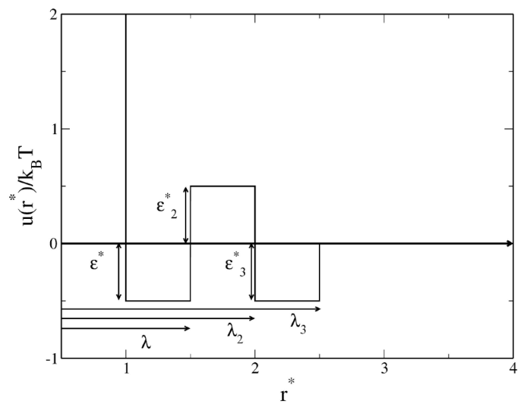
The depth of the first well 𝜖 is used to express the reduced temperature T ^* = k _B T /𝜖, where k _B is the Boltzmann constant, the particle diameter σ is used to reduce r*= r/σ, λ = λ/σ, and ρ* = ρσ ³; ρ is the particle number density. From Eq. (1), several cases can be considered depending on the values chosen for the interaction parameters. For example, Eq. (1) reduces to the well-known hard-sphere (HS) potential when 𝜖 = 𝜖 ₂ = 𝜖 ₃ = 0. We will consider the following three cases of Eq. (1): (a) the SW potential, defined by 𝜖 > 0 and 𝜖 ₂ = 𝜖 ₃ = 0; (b) the SWB potential, defined by 𝜖 > 0, 𝜖 ₂ > 0, and 𝜖 ₃ = 0; and (c) the SWBW potential, defined by the complete Eq. (1). In this way, SW fluids are characterized by a single well, SWB fluids by a well and a barrier, and SWBW fluids by two wells with a barrier in between.

SW fluid is probably the most studied DPF [²⁹,³²,³³,³⁵- ⁴⁰, ⁴², ⁴³, ⁴⁵, ⁵⁸, ⁶³, ⁶⁷, ⁷¹, ⁷³-⁷⁶]. Here we review its thermodynamic and structural properties, as a reference fluid. In particular, we explore its physical properties over an interval λ ∈ [1.5, 3] in steps of Δλ = 0.5. Note that λ = 1.5 is a typical value chosen in the context of simple liquids, while λ > 2.0 has been less studied.

We extensively studied different values for λ ₂ and of the SWB fluid; however, we present only those cases where a clear competition between microphase and macrophase separations seems to be observed. More precisely, we considered the following parameters for the SWB fluid: λ=1.25 and 1.5; λ ₂ = 2.0 and 3.0; and ∈ [0.1, 0.5]. For the SWBW fluid, the potential parameters used are: λ= 1.5; λ ₂ = 2; λ ₃ = 2.5; ∈ [0, 0.5]; and ∈ [0, 0.5].

In Gibbs ensemble simulations [⁴⁹, ⁷⁹], we initially placed 2048 particles with uniform distribution inside two cubic boxes of equal volume. Then, we carried out the following trial moves: displacement of particles in each box, volume change while the total volume remains constant, and particle exchange between the boxes. A Monte Carlo cycle randomly performs theses operations in the ratio 800:199:1, respectively. We used 2.5 × 10⁵ Monte Carlo cycles to equilibrate the system and 2.5 × 10⁵ production cycles. The acceptance ratio for both particle displacement and volume changes was fixed to 50%.

The phase diagram for the SW fluid was compared with results obtained using self-consistent Ornstein-Zernike approximation (SCOZA) [⁴⁰]. For SWB fluids exhibiting a liquid-vapor phase transition, we studied the microstructure near the critical point using MC computer simulations in N V T ensemble. We used 2048 particles, 2 × 10⁵ cycles to equilibrate the system, 2 × 10⁵ cycles to obtain statistics, and 50% acceptance ratio. Moreover, when the interaction is sufficiently long-range, phase coexistence disappears. In such a case, we focused on the microstructure at low temperatures.

Microstructure was studied by solving the Ornstein-Zernike (OZ) equation [⁵²], which defines the direct correlation function c( ) in terms of the total correlation function, h() = g() - 1, where g() is the radial distribution function. For homogeneous and isotropic fluids, the OZ equation takes the following form [⁵²],

To solve Eq. (2), a relation between c(r) and h(r) is required, which incorporates the information of the interaction potential and allows to close the set of equations. The most general closure relation is as follows:

where γ(r) = h(r) - c(r) is the indirect correlation function and B(r) is the bridge function [⁷⁷]. However, the form of B(r) is unknown and further approximations are required to find the solution to the OZ equation. In this work, we numerically solved Eq. (2) using the Ng method [⁷⁸] and assuming a particular choice for B(r). We used different closure relations to determine the regime of applicability, in terms of potential parameters, where they accurately describe the microstructure of the fluid. We used three types of conventional closure relations: PY, MSA, and HNC [⁵³-⁵⁵]; and two that incorporate thermodynamic selft-consistency: HMSA and RY [⁵⁶, ⁵⁷]. These relations can be expressed in terms of B(r) as follows:

PY

MSA

HNC

RY

HMSA

where u _a (r) is the attractive contribution to the interaction potential u(r) = u _r (r) + u _a (r) and u _r (r) is the repulsive contribution. In Eqs. (7) and (8), f(r) is a mixing function defined as f(r) = 1 - exp(-α(r)) and α is the mixing parameter. α is calculated by demanding thermodynamic self-consistency, which is estimated by equating the isothermal compressibility χ of fluid from the virial route Χ _u ^-1 = (∂BP/∂ρ) _T and the compressibility route Χ _c ^-1 = 1- ρ (q = 0), i.e., Χ _c ^-1 = Χ _u ^-1 [56, 57], where P is the pressure of the system and (q) is the Fourier transform of the direct correlation function.

Excess chemical potential μ is not reported, but can be determined during simulations with no additional cost by simply evaluating the following expression [⁴⁹]

where Δu is the energetic cost of inserting a particle in box 1, Λ is the de Broglie thermal length, and < … > represents an ensemble average. Similarly, μ ₂ in the second box can be easily evaluated. We also computed the pair correlation function and the pressure at coexistence. Both quantities can be used to test theoretical predictions based on the liquid state theory, such as the OZ Eq. (2) [⁵²].

The equation of state for discrete potential fluids of Eq. (1) can be determined using the following virial Eq. [³²]:

where λ _i denotes the discontinuity points of the potential and Δg(λ _i ) = g(λ _i ⁺ ) - g(λ _i ^- ) is the difference of the contact values of the radial distribution function at the discontinuity. In addition, this equation is exact. For an HS fluid, i = 0 and the summation contains only the term Δg(σ) = g(σ ⁺). Furthermore, the SW fluid involves Δg(λ) = g(λ ⁺) - g(λ ^- ), the SWB considers Δg(λ ₂) = g(λ ₂ ⁺) - g(λ ₂ ^-), and the SWBW includes the contribution Δg(λ ₃) = g(λ ₃ ⁺) - g(λ ₃ ^-).

3. Liquid-vapor phase diagram

3.1. SW fluid

Although phase coexistence of the SW fluid has already been studied in detail [²⁹,³⁹,⁵⁸-⁷⁴], we inspected the dependence on λ, as shown in Fig. 2. We show the phase diagram for different ranges of attraction: λ= 1.5, 2.0, 2.5, and 3.0; and observe that an increase in λ results in high coexistence temperatures. This can be explained as follows: when the thermal energy is not high enough compared to the well depth, the particles on average will be located in the region of the attractive well to minimize the free energy of the system. This is the driving force that generates the formation of well-defined particle domains, as discussed in Ref. [³²]. Thus, to avoid such particle agglomeration and to find the system within the fluid phase, thermal energy has to increase. In addition, the critical density does not change significantly with the interaction range. Furthermore, the data from the present simulation agree with estimates reported in the literature using Molecular Dynamics, GEMC [⁸⁰, ⁸¹] (data not shown), and the Self Consistent Ornstein-Zernike Approximation (SCOZA) [⁴⁰].

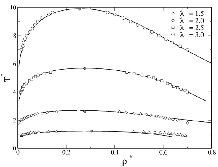
Figure 2 Liquid-vapor phase diagrams of SW fluids for λ = 1.5, 2, 2.5 and 3. Open symbols correspond to simulation data and lines to SCOZA results taken from [⁴⁰]. Closed circles indicate simulation results near the critical points. 

3.2. SWB fluid

To better understand the coexistence behavior of the SWB fluid phase, we define the following quantity: · 𝜖 ₂ /𝜖; which describes the repulsion strength in reduced units, 𝜖 is the energy unit and its reduced value is always 𝜖 ^* = 1.

In Fig. 3 we studied the effect of the repulsion strength, , on phase behavior; we use the following parameters for the potential: λ= 1.5 and λ ₂ = 2. We observed that the repulsion affects the critical values of density and temperature, these decrease as increases, the barrier tends to inhibit the phase transition. With the simulation study, we found that the phase transition is completely inhibited for > 0.8, we could observe that as the barrier height increases, the energy difference ΔE = + 𝜖 ^* also increases, thus forming an effective barrier that prevents the particles from falling into the potential well, as a consequence of thermal fluctuations. Therefore, high thermal energy is required to transfer particles from one well to another; this decreases the critical point as the barrier increases.

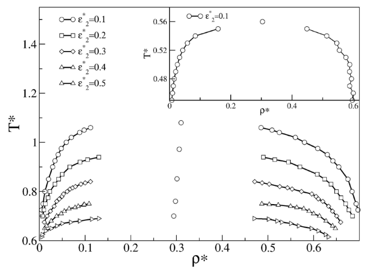
Figure 3 Liquid-vapor phase diagrams obtained with Gibbs ensemble simulations of SWB fluids for λ =1.5, λ ₂ = 2.0, 𝜖 ^* =1.0, varying = 0.1, 0.2, 0.3, 0.4, and 0.5. The inset shows the liquid-vapor phase diagram for λ = 1.25 and λ ₂ = 2, it only appears for 𝜖 ^* ≤ 0.1. The circle indicates the critical point and the lines are only a guide for the eye. 

We estimated the effective threshold barrier ΔE _t that completely inhibits the liquid-vapor transition and found that ΔE _t depends on height of and the repulsive range. For a short width repulsive interaction (Δλ = λ ₂ - λ ≲ σ/2) a higher barrier is required to inhibit the coexistence, if λ = 1.5 and λ ₂ = 2.0, a barrier height of = 0.8 can inhibit LV coexistence. However, for Δλ = λ ₂ - λ ≳ σ/2, a small barrier is required to promote cluster-phase formation and inhibit coexistence. The inset of Fig. 3 shows the phase diagram for the attractive and repulsive interactions at short- and long-range, respectively, also for λ = 1.25 and λ ₂ = 2, coexistence appears if ≤ 0.1. In the next section we discuss the structure properties to elucidate this behavior.

In addition, we observed that when the barrier height decreases below zero, the phase diagram shifts to higher temperatures (data not shown) because the barrier acts as a second well and particles can distribute in both wells, strongly favoring the phase transition. Theoretically, when studying the liquid-vapor phase diagram of SWB fluid using advanced approaches, such as SCOZA, the standard procedure described in Ref. [⁴⁰] fails to converge numerically when an additional barrier in the interaction potential is explicitly considered. However, further considerations of the fluid coexistence of DPFs can be evaluated using SCOZA, which is discussed elsewhere.

3.3. SWBW fluid

In the case of SWBW fluid, a secondary attractive well is added to the SWB potential and the interaction ranges are fixed at λ =1.5, λ ₂ =2.0, and λ ₃ = 2.5. To investigate phase coexistence of fluids with competing potential, we analyzed the following two interesting cases: increasing the repulsive contribution, and increasing the attractive strength of the second well, separately. The attractive and repulsive strengths are tuned as follows, in two cases: (1) 𝜖 ^* = 1.0 and = 0.1 are fixed and the barrier height is varied; and (2) 𝜖 ^* = 1.0 and = 0.5 are fixed and is varied.

Figure 4 shows the results of the first case, where the barrier height is increased. We found that when the barrier height increases, the repulsive contribution shifts the coexistence region towards low temperatures region. However, coexistence of SWBW fluids is observed at higher temperatures than in the case of SWB fluids, thus the attractive contribution favors liquid-vapor coexistence. Therefore, the second well increases the effective attractive range. However, the barrier and the second well generate an effective barrier height, i.e., + , which inhibits coexistence. As the barrier height increases, the system needs more energy to attain coexistence, which is reflected in a low critical temperature with increasing barrier height.

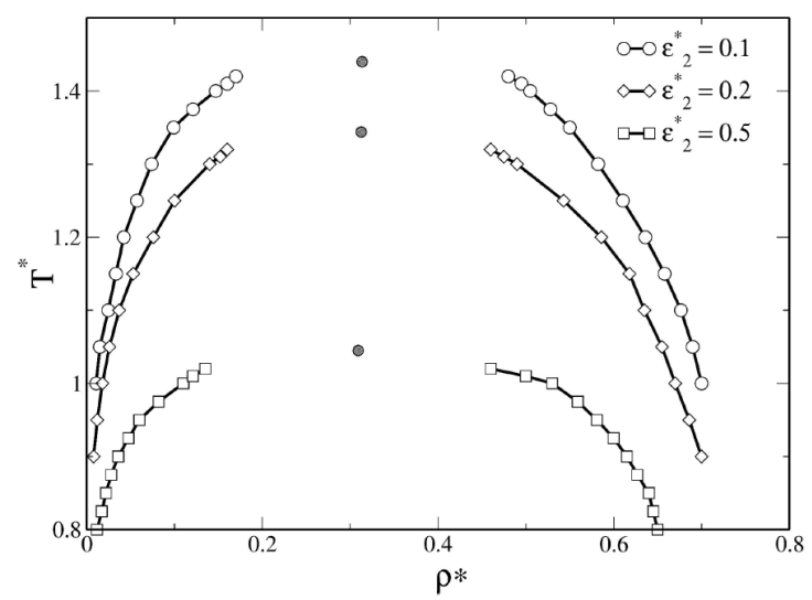
Figure 4 Phase diagram of SWBW fluids. The values of 𝜖 ^* = 1.0 and = 0.1 are fixed. The effect of increasing the barrier height is studied. The values of the barrier height are: = 0.1, 0.2, and 0.5. These results were obtained using GEMC and the dark circle indicates the critical point. 

To examine the effect of the second well, we considered three values of well depth = 0.1, 0.2, and 0.3. In this case, coexistence shifts toward higher temperatures as well depth increases, Fig. 5, indicating that the second well promotes LV coexistence. In both SWBW cases, macrophase separation appears for any well depth or barrier height. The presence of a second well increases the effective interaction range and well depth.

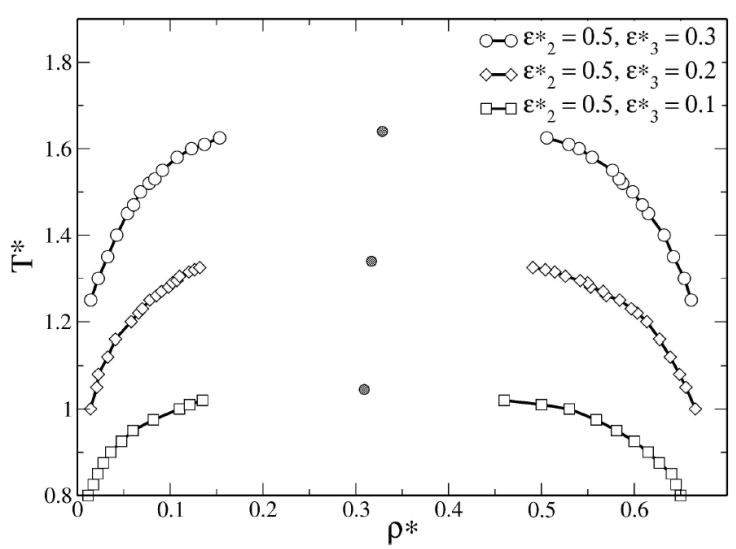
Figure 5 Phase diagram of SWBW fluids, the values of 𝜖 ^* = 1.0 and = 0.1 are fixed, and the effect of increasing the well depth is studied. The values of the well depth are = 0.1, 0.2, and 0.3. The results were computed using GEMC and the dark circle indicates the critical point. 

Finally, in Table I we present the critical values for each discrete potential fluid studied in this section. Critical temperatures and densities were obtained from the law of rectilinear diameters [⁵⁰], since the critical values cannot be calculated directly from GEMC simulation.

Table I Critical densities and temperatures for SW, SWB, and SWBW fluids. 

Type	𝜖 2 *	𝜖 3 *	λ	λ 2	λ 3	T c *	ρ c *
SW	0.0	0.0	1.5	2.0	2.5	1.226	0.304
SW	0.0	0.0	2.0	2.0	2.5	2.624	0.274
SW	0.0	0.0	2.5	2.0	2.5	5.67	0.276
SW	0.0	0.0	3.0	2.0	2.5	9.980	0.255
SWB	0.1	0.0	1.5	2.0	2.5	1.080	0.310
SWB	0.2	0.0	1.5	2.0	2.5	0.972	0.306
SWB	0.3	0.0	1.5	2.0	2.5	0.851	0.301
SWB	0.4	0.0	1.5	2.0	2.5	0.760	0.297
SWB	0.5	0.0	1.5	2.0	2.5	0.700	0.294
SWB	0.1	0.0	1.25	2.0	2.5	0.559	0.3035
SWBW	0.1	0.1	1.5	2.0	2.5	1.440	0.313
SWBW	0.2	0.1	1.5	2.0	2.5	1.344	0.312
SWBW	0.5	0.1	1.5	2.0	2.5	1.045	0.309
SWBW	0.5	0.2	1.5	2.0	2.5	1.339	0.316
SWBW	0.5	0.3	1.5	2.0	2.5	1.640	0.328

4. Structure

Cluster formation was studied using short attractive and large repulsive potentials. Here we discuss the structural properties of SW, SWB, and SWBW fluids. The structure factor S(q) is computed using MC simulation in NVT ensemble and the OZ equation. For each case, we studied the structure in the equilibrium region and near the critical point. We explored a wide range of values of parameters defining the interaction potential, i.e., the strength and range of each contribution.

We considered two conditions on the structure factor for cluster formation [⁵-⁷, ⁹]: (1) a low-q peak value located at , i.e., the cluster-cluster peak. This peak corresponds to a mean distance between clusters ~ 2π= and characterizes the repulsive interaction between them. (2) A main high-q peak value, namely, monomer-monomer peak, located at (2π/σ), which corresponds to the mean distance between monomers within a single cluster (with q _c < q _m ).

For the SW fluid, we analyzed the structure for each value of λ studied in Sec. 3, however, we show only the cases for λ = 2.5 and 3.0, because these values are less studied and, in addition, we found an unusual structural behavior. For λ ≤ 2.0, the structure has been reported in Ref. [³², ³⁴] with a typical structural behavior of a homogeneous fluid. Figure 6 shows S(q) of the SW fluid for λ =2.5 and 3.0 (inset), the formation of a peak at is observed. For λ = 2.5, the peak is localized at ~ 5.98, which corresponds to r ~ 1.05; and for λ = 3.0, the peak is localized at ~ 5.2, which corresponds to r ~ 1.2. In these two cases, the height of the peak at is slightly smaller than that of the peak at , indicating that the structure is sensitive to the interaction range, and that a singular behavior appears for large values of λ. In the system, there is a characteristic length l _c = 2π =, where l _c >σ. A peak at is close to a peak at and this behavior corresponds to the formation of well-defined domains or dimers, promoting the LV coexistence.

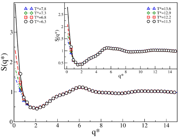
Figure 6 Structure factor S(q∗) of SW fluids for 𝜖 ^∗ = 1.0 and λ =2.5, at ρ ^∗ = 0.225. In the inset 𝜖 ^∗ = 1.0 and λ =3.0. Symbols represent MC simulation data and lines represent OZ-HMSA. 

For the SWB fluid, we investigated the same values of λ and 𝜖 ^* studied in Sec. 3. We first present the results for a short-range attractive interaction (λ = 1.25) and then a medium-range repulsive interaction, where the effect of increasing barrier is studied. Figure 7 shows S(q) for = 0.1, where the value of S(q ^* → 0) increases as temperature decreases, this is a typical thermodynamic behavior in the liquid-vapor transition. However, the structure factor for = 0.3 exhibits an unusual peak at low-q, which increases with decreasing temperature. This behavior is characteristic of cluster-phase formation. Thus, for this interaction range, LV coexistence disappears and a cluster-phase formation appears. This behavior is elicited by a slight increase in the barrier height.

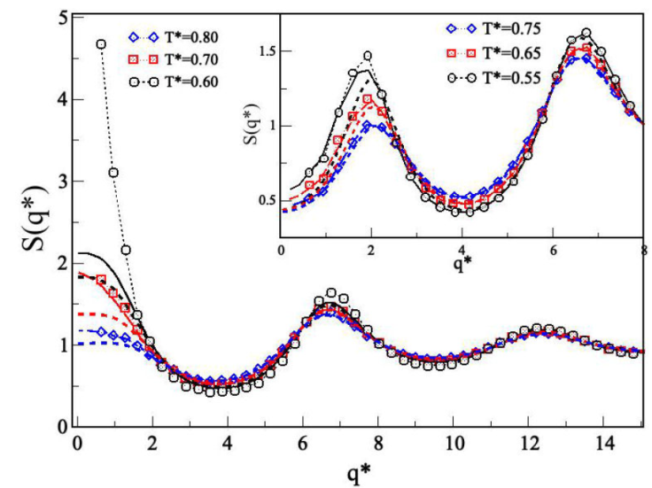
Figure 7 Structure factor S(q*) of SWB fluids for 𝜖 ^* = 1.0, = 0.1, λ =1.25, and λ ₂ =2 at ρ ^* = 0.275. In the inset 𝜖^∗ = 1.0, = 0.3, λ =1.25, and λ ₂ =2. Symbols represent MC simulation data, lines represent OZ-HMSA, in the outset, the solid line is computed by PY, and dashes lines are computed from Santos et al work [²⁵]. 

Figure 8 shows S(q) for the system with medium-range attractive and medium-range repulsive interactions, i.e., λ ₁ = 1.5 and λ ₂ = 2.0, with = 1.0, and = 0.5 and 0.7 (inset). We explored the cases where ∈ [0.1, 0.7], nevertheless, we found that ≤ 0.6, the fluid has a typical behavior, i.e., S(q ^* → 0) increases as the temperature decreases and no low-q peak appears. For this reason, we show two representative cases ( = 0.5 and 0.7). For = 0.7, a slight peak formation appears at q ^* < 2 and this peak is more evident as the temperature increases. Thus, a high barrier is required to find a cluster-phase, which coincides with the fact that LV coexistence disappears. In Figs. 7 and 8, we observe that the data computed from Santos et al. work, in most cases, reproduces main peak behaviour at q ^* ~ 2π, but fail to q ^* ≤ 2, this is because, for this cases, the rational functions approximation method does not reproduce the contact values of the radial distribution function.

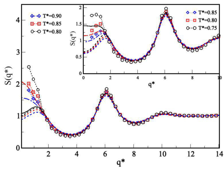
Figure 8 Structure factor S(q∗) of the SWB fluids for 𝜖^∗ = 1.0, = 0.5, λ =1.5, and λ₂ = 2, at ρ ^∗ = 0.275. In the inset 𝜖^∗ = 1.0, = 0.7, λ =1.5 and λ₂ =2. Symbols represent MC simulation data, lines represent OZ-HMSA, the solid lines are computed by PY, and dashes lines are computed from Santos et al work [²⁵]. 

Figure 9 shows the last case of SWB fluid, corresponding to a medium-range attraction and a long-range repulsion: λ ₁ = 1.5 and λ ₂ = 3, respectively. We explored ∈ [0.1, 0.5], but only two significant values were shown: = 0.1 and 0.2 (inset). We found that liquid-vapor coexistence disappears even for a small repulsive barrier. We observed cluster formation for any barrier height, which results from long-range repulsive interactions. A peak at low-q values was observed, i.e., we found an S(q _c ) at q _c representing cluster formation, and this peak appears for any temperature value.

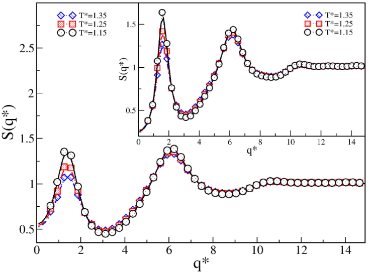
Figure 9 Structure factor S(q ^* ) of SWB fluids for 𝜖^∗ = 1.0, = 0.1, λ =1.5, and λ ₂ =3, at ρ ^* = 0.250. In the inset 𝜖^∗ = 1.0, = 0.2, λ =1.5, and λ ₂ =3. Symbols represent MC simulation data and lines represent OZ-HMSA. 

In the case of the SWB fluid, a clear relationship was observed between the cluster-phase formations and the strength and range of interaction. After a comprehensive study, we found a relevant behavior, shown in Fig. 10. We studied the microphase and macrophase formations in terms of λ _r and , and explored the region in which LV coexistence rules and the region in which cluster formations or microphase appears; thus, we determine the boundary between phases. The white dots in Fig. 10 correspond to the macrophase or LV coexistence, and the black dots correspond to the region where coexistence is inhibited and microphase appeared. We explored several temperatures near and below the critical temperature, in Fig. 10 we show two representative systems: SWB1 with λ = 1.5 and λ ₂ = 2.0, and SWB2 with λ = 1.25 and λ ₂ = 2.0. In this study, we set an exponential fit for the boundary between both regions. For the SWB1 case with λ _r = 0.33, LV coexistence is inhibited for > 0.7, whereas for the SWB2 case with λ _r = 0.6, LV transition is inhibited for > 0.2. In addition, for the extreme case, when λ _r ≥ 1 there are microphase separations even with barrier height < 0.1.

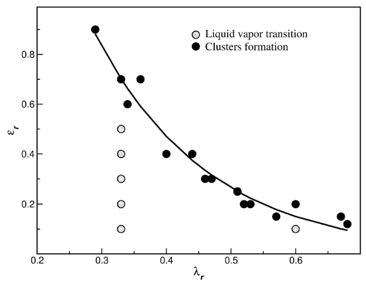
Figure 10 Schematic view of cluster-phase formations and macrophase separations as a function of the range and strength of the interaction. 

Finally, the competing effect on the structural properties for the SWBW case is discussed. Here we considered the following medium interaction ranges: λ = 1.5, λ ₂ = 2.0, and λ ₃ = 2.5. As in Sec. 3, interaction ranges were fixed with varying barrier height and second well depth. In the first case, the depth of the attractive contribution is fixed and the height of the repulsive contribution is varied. In the second case, the second attractive contribution is varied and the repulsive contribution is fixed. For both cases, we found typical fluid phase behavior. Figures 11 and 12 show the structure factors: the presence of the second well promotes macrophase separations regardless of the depth of the second well, which is in agreement with the results presented in Sec. 3. Here, the effects induced by the barrier to favor microphase separations have vanished.

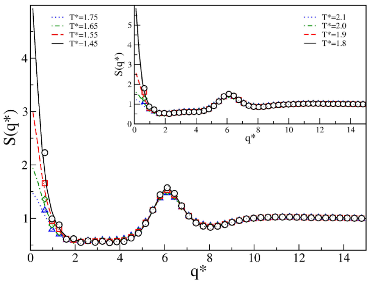
Figure 11 Structure factor S(q*) of SWBW fluids for 𝜖^∗ = 1.0, = 0.5, = 0.3, λ =1.5, λ ₂ =2 and λ ₃ = 2.5 at ρ ^* = 0.275. In the inset 𝜖^∗ = 1.0, = 0.3, = 0.2 λ =1.5, λ ₂ =2 and λ ₃ = 2.5. Symbols represent MC simulation data, lines represent OZ-HMSA and solid lines in both graphics are computed by PY. 

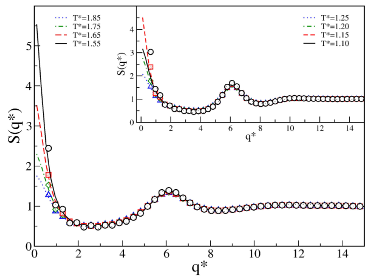
Figure 12 Structure factor S(q⁄) of the SWBW fluids for 𝜖^∗ = 1.0, = 0.3, = 0.1 λ =1.5, and λ ₂ =2 and λ ₃ = 2.5, at ρ ^* = 0.275. In the inset 𝜖^∗ = 1.0, = 0.1, = 0.1, λ =1.5, λ ₂ =2 and λ ₃ = 2.5. Symbols represent MC simulation data, lines represent OZ-HMSA and the solid line in the inset was computed by PY. 

Structural studies use many closure relations, such as PY, MSA, HNC, HMSA, and RY, to solve the OZ equation. In this study, for SW and SWBW fluids, RY closure is not a good approximation to solve the OZ equation, because it is not convergent for most densities, which is consistent with previous research [⁸²]. The MSA closure converges in most cases, but the results do not agree with simulation data. Conversely, PY, HNC and HMSA converge for temperatures above the critical point, and the results agree with MC data. However, HNC and HMSA do not converge near the critical point.

In the case of SWB fluid, PY converged only around the critical point, however it is not a good approximation. No-Notably PY, HNC, and HMSA converged above the critical point, and are considered the best approximations; nevertheless, for q ^* → 0 differences between closures results are observed. In cases where LV phase separation does not appear, most of the closure relations converge, but there are differences at low temperatures. However, PY, HMSA, and HNC approximations reproduce the simulation data and the second peak at q-low.

5. Conclusions

For simple attractive interactions, such as SW fluids, the interaction range plays a primary role in microphase and macrophase separations. Besides, the attractive potential promotes LV coexistence, which appear at higher temperatures with increasing interaction range. However, the results show that increasing the interaction range favors the formation of microphases, in particular for λ ≥ 2.5, with the appearance of domains or dimers formation.

Competing interactions, as in SWB fluids, can give rise to microphase and macrophase separations that do not appear in simple fluids. In this case, the interaction range plays a primary role in microphase and macrophase separations and interaction strength. We found that for short-range attractive and long-range repulsive interactions, LV coexistence is inhibited and microphase separation appears when the barrier height is increased. Besides, poor LV coexistence is related to cluster-phase formations. A similar effect is shown in the case where the attractive interaction is medium-range and the repulsive interaction is long-range. However, in this case, the cluster-phase formations are independent of barrier height. In addition, in both SWB cases, cluster formation is related to the absence of LV coexistence. Nevertheless, for medium-range attractive and repulsive interactions, a large barrier height is required to observe a trace of cluster-phase formation. In this case, macrophase separation dominates and LV coexistence appears for several values of barrier height. In SWBW fluids, the second well favors macrophase separations, and LV coexistence appears regardless of barrier height. Thus, long-range attractive interaction inhibits cluster-phase formations. Finally, we showed that DPFs are useful to study the effects of attractive and repulsive potentials on LV coexistence and cluster formations. Furthermore, we were able to determine the effect of the range and strength of the interaction on microphases and macrophases, separately.