




 nueva página del texto (beta)
 Inglés (pdf)
 Artículo en XML
 Referencias del artículo

 Traducción automática
 Enviar artículo por email
 Citado por SciELO
 Similares en
SciELO

 Permalink


1. Introduction
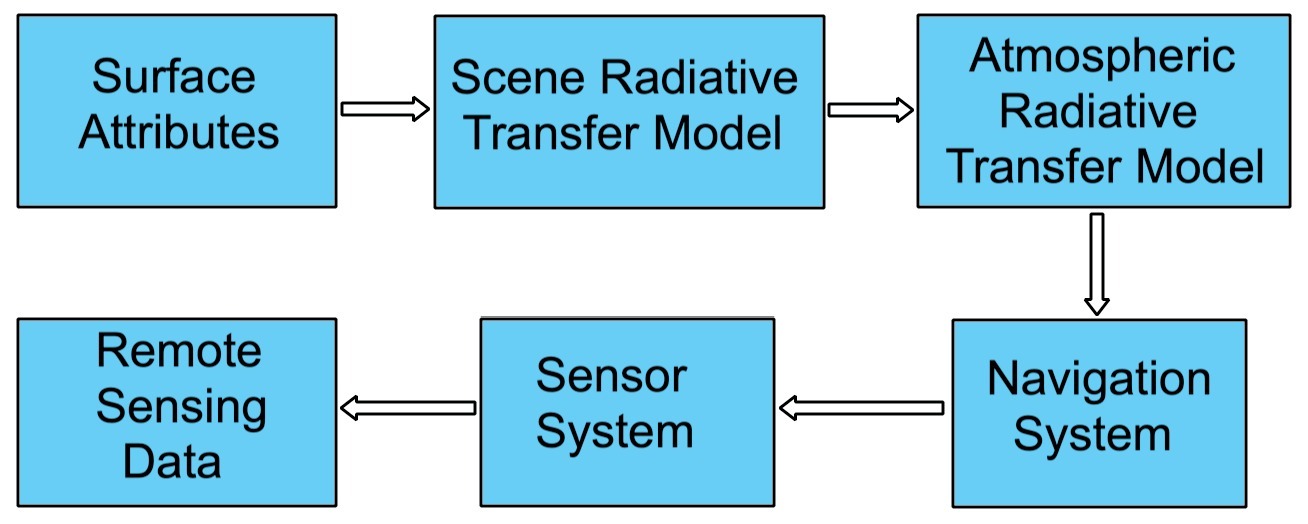
An optical Remote Sensing system can be separated into five subsystems (Liang et al., 2012), Figure 1: The scene radiative transfer model, the atmospheric radiative transfer model, the navigation system, the sensor system, and the mapping and binning system. The scene radiative transfer model describes the interaction between the target surface (i.e. area of interest or area to be studied) radiative signals and the surface characteristics (i.e. spectral signatures, adjacency effects,etc). The atmospheric radiative transfer model characterizes the effects (i.e. distortions) of the atmosphere on surface radiative signals that are received by the satellite sensors. The navigation system involves the elements needed to keep the satellite in a certain orbit and to keep the optical sensor stable (i.e. attitude control subsystem). The sensor system includes the sensor spectral response (i.e. wavelength sensitivity), spatial response (i.e. Instantaneous Field of View), band division (i.e. bands to be used), noise treatment (i.e. noise filtering or denoising), and digital processing (i.e. resampling, compression,etc). Some authors (Liang et al., 2022) add the mapping and binning system after the sensor system; since it is related to digital processing, we will omit it here for the sake of simplicity.
In this article we will mainly focus on the atmospheric radiative transfer theory (Buglia, 1986) since it allows to model the interaction between the sun light,the characteristic of the earth surface and the signals received by the satellite sensors (although other approximate AC methods that do not rely on this theory have been proposed). This interaction model is a key factor to retrievequantitative remote sensing analysis of the surface characteristics using satellite imagery. The two main contributors to image degradation because of the atmosphere in remote sensing are scattering and absorption(Richards, 2022). In general scattering has an additive effect (Zhang et al., 2010; Chavez, 1996) while both the scattering and absorption have a multiplicative effect on the image (Chavez, 1996). The additive scattering effect can be seen as a haze in the image, so basic atmospheric correction such as DOS1 attempts to correct for additive scattering resulting in a dehazed image (Chavez, 1988). There exist other methods that can correct for both the additive and the multiplicative effect of atmosphere on satellite imagery.
The purpose of this paper is to present a global overview of the methods currently available and mentioned in the literature to perform AC on any of these three cases. Section 2 includes the methodology followed to select the articles included in this review, the inclusion and exclusion criteria, search strategy and outcomes, data abstraction and synthesis. Section 3 includes the results obtained for each category of AC used by surface type. Since AC for inland waters and oceans share some common principles, they will be discussed on the same section, mentioning the differences that make them two different application types. Section 4 discusses some potential factors needed to consider when selecting the appropriate AC algorithm, as well as current trends in AC. Finally, section 5 presents some conclusions regarding the area of AC.
1.1. Is Atmospheric Correction Neccesary?
Atmospheric correction may not always be necessary. In general, it can be ignored if just qualitative remote sensing is to be done. Jensen, 2015, mentions that certain types of classification and change detection may not need atmospheric correction. Land use/cover only needs qualitative analysis so AC can be omitted since we are not interested on spectral (radiometric) properties of the area of interest (Lwin et al., 2012). If quantitative Remote Sensing is to be done (Jensen, 2015; Liang, 2003) then AC is an essential pre-processing step. For example, it is usually necessary to perform AC when the remote sensing data are biophysical parameters to be extracted from water bodies (e.g., chlorophyll a, suspended sediment, temperature) or vegetation (e.g., biomass, leaf-area-index, chlorophyll, percent canopy closure). If the data are not corrected, the subtle differences in reflectance among the important constituents may be partially or totally lost.
1.2. Should Atmospheric Correction be applied independently?
There exist two main commercial satellites where images for remote sensing analysis can be downloaded: Landsat and Sentinel. Landsat offers two image levels, where each level offers the following processing features:
Landsat level 1: This level offers three different options named L1TP (Terrain Precision Correction), L1GT (Systematic Terrain Correction), L1GS (Geometric Systematic Correction). L1TP is radiometrically calibrated and ortho-rectified, being the most used image type for Time Series analysis (Bhandari et al., 2012).
Landsat level 2: Historically, most Earth Observation images have been provided to the users in terms of calibrated DN, where each user individually must apply the pertinent radiometric calibration and perform atmospheric correction to retrieve earth (land or water) surface reflectance. Level 2 images provide surface reflectance estimation by applying the atmospheric correction. The Land Surface Reflectance Code (LaSRC) is the atmospheric correction algorithm of Landsat 8, as currently implemented at United States Geological Survey Earth Resources Observation and Science (USGS EROS). This algorithm is designed to model the atmospheric conditions at the time of the satellite’s overpass, utilizing ancillary data such as ozone levels, water vapor content, carbon dioxide, aerosol distribution, and surface pressure (Adhikari et al., 2025). The mean percent absolute error for Level-2 surface reflectance data ranges from 3.3% to 10% (Teixeira, 2020).
On the other hand, Sentinel offers the following processing levels, Sentinel-2 User Handbook:
Level 0: Not released to users
Level 1A: Not released to users
Level 1B: It is the first public product. It comprises radiometric corrections (dark signal, pixels response non-uniformity, crosstalk, defective pixels, restoration, and binning for 60m bands); and an enhanced physical geometric model appended to the product but not applied (Baillarin et al., 2012).
Level 1C: The Level-1C product results from using a Digital Elevation Model (DEM) to project the image in cartographic coordinates. Per-pixel radiometric measurements are provided in Top Of Atmosphere (TOA) reflectances with all parameters to transform them into radiances.
Level 2A:The Level-2A product provides Bottom Of Atmosphere (BOA) reflectance, or surface reflectance images, derived from the associated Level-1C products. Sen2Cor is the processor for Sentinel-2 Level 2A product generation and formatting; it performs the atmospheric, terrain and cirrus correction of Top Of Atmosphere Level 1C input data. Sen2Cor creates Bottom Of Atmosphere, optionally terrain and cirrus corrected reflectance images; and additionally, Aerosol Optical Thickness and Water Vapor, something that could only be estimated from Sentinel 2 observations. The Sentinel 2 MSI instrument has the spectral band 9 located in the water vapor absorption region (Central Wavelength: 945 nm) and so it is appropriate for the water vapor correction, while Landsat 8 OLI lacks this feature (Doxani et al., 2018).
While Level 2 images from both Landsat and Sentinel can provide reasonably good atmospherically corrected images, for many applications it is required more accuracy as shown by Ni et al., 2025, where FLAASH AC algorithm applied to Level 1 images outperforms Level 2 data for identifying soil salinization. Zhou et al., 2021, showed also that several improvements can be done for both Landsat and Sentinel images when optimized AC algorithms are applied to level 1 products. Also, since water surface reflectance can be more challenging to be estimated, more specialized algorithms must be used to retrieve water leaving radiance with good accuracy (Pahlevan et al., 2021). The decision to use either level 1 or Level 2 images depends upon the application and the accuracy level required for the specific final application. Level 2 images can be good enough for an initial screening of the region of interest, while Level 1 images with custom AC should be considered if high accuracy level is required (i.e. stable surface reflectance accuracy) or a challenging complex surface is being studied (i.e. inland or coastal waters).
1.3. Types of Atmospheric Correction
Atmospheric Correction (AC) aims to retrieve surface reflectance (either land reflectance or water reflectance). There are two main types of atmospheric correction approaches, which differ depending on the units of the result. According to some authors like (Jensen, 2015; Hadjimitsis et al., 2004), AC algorithms can be grouped into two types:
Absolute Atmospheric Correction (corrections that lead to surface reflectance)
Relative Atmospheric Correction (corrections that may or may not produce surface reflectance)
1.3.1. Absolute Atmospheric Correction
In this type of correction, the goal is to retrieve the surface reflectance as if it was measured from the earth surface. There exist several methods to perform this type of AC, some of them make use only of the image itself and the image meta data, they are called Image Based Methods, while the most sophisticated need auxiliary information such as the aerosol optical depth (AOD) among other atmospheric parameters. These methods usually rely on the use of any Radiative Transfer Code (i.e. 6S, MODTRAN, LibRadtran, SMAC) (Hadjimitsis et al., 2004).
1.3.2. Relative Atmospheric Correction
Relative AC does not lead usually to surface reflectance. Its purpose is to normalize multitemporal images so that the corrected images appear as if they were taken under the same atmospheric and illumination conditions (Schott et al., 1988). The normalization procedure can also be done using reflectance units, in this case the image will be normalized using reflectance units. The procedure described in (Schott et al., 1988), is similar to Histogram Matching; given a reference histogram shape (of a reference image), the objective is to transform another image (image to be normalized) to match as close as possible the reference image histogram doing a linear transformation.
1.4. Applications of AC by surface type
As mentioned earlier, AC can be done to retrieve surface reflectance either in land or water (which cover the entire earth surface). There existAC algorithms that are designed to be applied in different surface types. The three big categories are:
Atmospheric correction for land use
Atmospheric correction for inland waters (i.e. lakes, rivers, coasts)
Atmospheric correction for oceans (ocean-color)
Before 2018, the reference of the state-of-the-art algorithms for AC was very scatter. Fortunately, in 2018 the Atmospheric Correction Inter-comparison eXercise (ACIX) was created with the idea of evaluating and comparing different AC algorithms, many of them already implemented in commercial processors. The aim of the ACIX is to analyze the Surface Reflectance (SR) products of various state-of-the-art atmospheric correction (AC) processors. The Aerosol Optical Thickness (AOT) and Water Vapor (WV) are also examined in ACIX as additional outputs of AC processing (Doxani et al., 2018; Doxani et al., 2023). On the other hand, The Atmospheric Correction Intercomparison Exercise (ACIX-Aqua), a joint NASA - ESA effort, was initiated to enable an evaluation of eight state-of-the-art atmospheric correction (AC) processors available for Landsat-8 and Sentinel-2 data processing. Over 1000 radiometric matchups from both freshwaters (rivers, lakes, reservoirs) and coastal waters were utilized to examine the quality of derived water reflectance (Pahlevan et al., 2021). The recommendations given by the ACIX initiative were also considered for the evaluation of the articles presented in this review. The ACIX initiative provides a good reference for developers and researchers on the strengths and weaknesses of the algorithms presented in this comparison exercise. Besides the algorithms presented in the ACIX initiative, some other recent works are also mentioned, some classical AC algorithms are also reviewed since some of them (i.e. DOS, QUAC, FLAASH) are still used and have even been improved over time, such as the DOS algorithm (Zhang et al., 2010).
2. Methodology
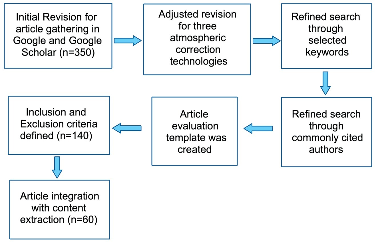
Figure 2 shows the stages followed during this review:
2.1. Inclusion and Exclusion criteria
This study included research articles involving atmospheric correction for land application, atmospheric correction for inland waters, atmospheric correction for oceans and aerosol optical depth retrieval published in peer-reviewed publications in English after mainly 2014. Articles published before 2014 were also considered when they are relevant on a specific topic, some of them were mentioned on these newer articles or are relevant to understand the evolution of any specific development, algorithm or proposal (i.e. recall Radiative Transfer Theory dates from 1960). It is worth to mention that the work of some authors is still relevant or frequently cited even when some of their work was published in the late 80s or even before. Conference papers were allowed while they were relevant to the state-of-the-art since it is logical to assume that sometimes very recent work isfirst published in conferences before jumping into journals. Some textbooks were also included as the first references since they provide a basic understanding on many topics. In general, the first inclusion criteria were the following:
Less than 10 years of being published
Commonly cited authors (even if their work was older than 10 years)
Articles with more than 10 years were also included in cases where they are still relevant or important to understand current developments or topics
Articles related tothe ACIX initiative, since they are considered as state-of-the-art because of the evaluation framework
Suggestions provided by the ACIX initiative to evaluate the selected articles.
The exclusion criteria were the following:
Studies involving hyperspectral imagery
Papers focused specifically on feature extraction in Remote Sensing images
Papers of more than 10 years presenting methods not currently relevant
Papers of not very common platforms (i.e. satellite types). On this regard, it was preferred to include papers using NASA or ESA satellite imagery. Exceptions were made, however.
Conference proceedings were mostly excluded, although a few recent articles with relevant topics were included as a reference (e.g. those ones focused on Machine Learning).
2.2. Search strategy and outcomes
A combination of keywords listed in Table 1, connected using Boolean operators (and/or), yielded around 350 articles during the initial database (Google and Google Scholar) search. First, these articles were screened based on title and abstract for the following exclusion criteria: papers of more than 10 years with no currently relevant content, conference proceedings of more than 10 years and languages other than English, resulting in 210 being excluded. The 140 remaining articles were subsequently screened based on their partial content reading. At the end 97 of these 140 articles were selected because of their content relevance and meet the inclusion criteria.
Table 1. Main keywords used to search for articles
| Keywords | |
|---|---|
| Radiance and Reflectance | Pseudoinvariant areas |
| Algorithms | MODIS |
| Atmospheric Correction | Radiative Transfer |
| Absolute | Dark Objects |
| Relative | Landsat |
| Inland Waters | Transmittance |
| Aerosol Optical Depth | Bio-Optical Model |
| Deep Learning | Machine Learning |
| Scattering and Absorption | Rayleigh Reflectance |
| Land Surface Reflectance | Water Leaving Radiance |
2.3. Quality Evaluation
In the evaluation template, a questionnaire was prepared with the following questions, based on the CRAAP method (Currency, Relevance, Authority, Accuracy, Purpose), to prioritize recent quality research papers. The questions in the template were the following:
Reason for selection (Title, abstract, keywords)
Publication date less than 10 years (exceptions allowed) (Yes or No)
Article fully related to AC methods (Yes or No)
Results verifiable (Yes or No)
Metrics clear (Yes or No)
Author frequently cited (Yes or No)
Even when some questions may be subjective, it was helpful to evaluate from a quantitative point of view the content of the article. Other criteria evaluated through a questionnaire were:
2.4. Data extraction
Selected articles were reviewed thoroughly, and data were extracted to systematically synthesize the information pertinent to the scope of this review. The extracted details are categorized and summarized in Appendix A, with the Results Section providing more detailed information about the individual categories. Table 2 lists the journals and conference proceedings in which the articles re-viewed were published.
Table 2. Journals of selected articles.
| Journal | Impact Factor | Publisher | Articles Included |
|---|---|---|---|
| Remote Sensing of Environment | 13.85 | Elsevier | 15 |
| Remote Sensing | 5.34 | MDPI | 40 |
| International Journal of Applied Earth Observation and Geoinformation | 7.67 | Elsevier | 2 |
| Urban Climate | 6.663 | Elsevier | 1 |
| International Journal of Geo-information (ISPRS) | 3.099 | MDPI | 1 |
| Journal of Geophysical Research: Atmospheres | 5.22 | AGU | 7 |
| International Journal of Remote Sensing | 3.531 | Taylor and Francis | 6 |
| IEEE Transactions on Geoscience and Remote Sensing | 8.125 | IEEE Xplore | 5 |
| IEEE International Geoscience and Remote Sensing Symposium (IGARSS) | 3.5 (IS) | IEEE Xplore | 4 |
| ISPRS Journal of Photogrammetry and Remote Sensing | 11.774 | Elsevier | 3 |
| Atmosphere | 3.110 | MDPI | 1 |
| Applied Optics | 1.905 | Optica Publishing Group | 5 |
| Canadian Journal of Remote Sensing | 2.13 | Taylor and Francis | 1 |
| Sustainable Environment Research | 3.99(IS) | Springer | 1 |
| Applied Geomatics | 2.357 | Springer | 1 |
| Journal of Geographic Information System | 1.56 | Scientific Research | 1 |
| International Journal of Image Processing | 6.82(CI) | International Journal of Image Processing | 1 |
| Photogrammetric Engineering and Remote Sensing | 0.96(IS) | American Society for Photogrammetry and Remote Sensing | 1 |
| Revista de Teledetección | 0.75(IS) | Asociacion Espanola de Teledeteccion | 2 |
| International Conference on Computational Intelligence and Multimedia Applications | N/A | IEEE | 1 |
| Sensors | 3.576 | MDPI | 1 |
| International Conference on Advanced Computing and Communication Technologies | 0.247(SJR) | Conference Publishing Services | 1 |
| Living Planet Symposium | N/A | Living Planet Symposium | 1 |
| Journal of Quantitative Spectroscopy & Radiative Transfer | 2.3 | Science Direct (Elsevier) | 1 |
| Geophysical Research Letters | 8.9(CI) | AGU | 1 |
| Journal of the Indian Society of Remote Sensing | 2.5 | Springer | 1 |
| Applied Sciences | 2.7 | MDPI | 3 |
| Journal of the Atmospheric Sciences | 3.1 | AMS | 1 |
| Boundary-Layer Meteorology | 4.3 | Springer | 1 |
| Critical Reviews in Environmental Science and Technology | 11.4 | Taylor and Francis | 1 |
| Algorithms | 2.0 | MDPI | 1 |
| Frontiers in Marine Science | 3.0 | Frontiers | 1 |
*IS: Impact Score, **SJR: Scimago Journal Rank ***CI: Citation Impact
3. Results
The primary goal of this review is to present a global perspective of the algorithms used for AC to retrieve surface reflectance either on land or water. As explained above, atmospheric correction is one of the most important preprocessing steps, particularly in Quantitative Remote Sensing (Liang, 2003). Depending on the type of surface to be analyzed and its location, there are different atmospheric correction algorithms that can be divided into the following three subgroups and of which the research on the state of the art was carried out:
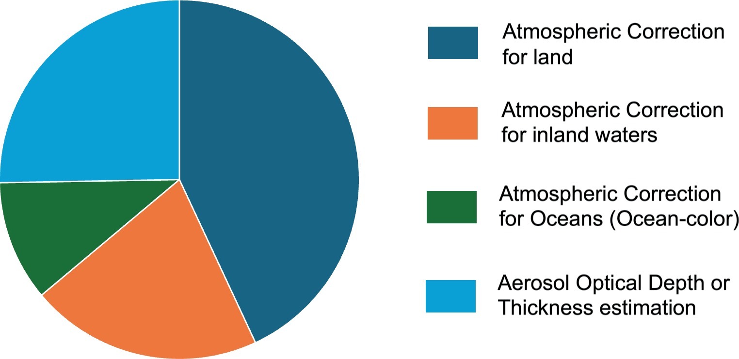
Additionally, a search for methods and algorithms was carried out to estimate the optical thickness of aerosols (AOD), since it is known that this is the variable that has the most important impact on the accuracy achieved with atmospheric correction algorithm (Hadjimitsis & Clayton, 2009). Figure 3 shows the proportion of the number of papers found in each area. In the following subsections an overview of each of these areas is given.
3.1. Land Atmospheric Correction
First, we will describe the basic theory for surface reflectance retrieval in the case of a land surface, assuming the Lambertian case, considering a Lambertian reflectance as the property that defines an ideal "matte" or diffusely reflecting surface.
3.1.1. Radiometric Calibration for Landsat Images (Basic Conversions)
Radiometric Calibration refers to the processof converting the digital numbers recorded by satellite imaging systems into physical units. A satellite image is captured in raw binary format also called Digital Numbers (DN). Each pixel has an original brightness value (Jensen, 2015). Radiometric calibration converts the digital numbers (DN) of the image pixels to physical units, such as radiance or reflectance. Several methods have been developed to perform radiometric calibration in satellite sensors. Before launching, sensors are calibrated to comply with international standards, nevertheless such calibration degrades over time, and a recalibration process must be conducted to ensure that the acquire data is accurate. One of the most popular methods for recalibration is based on using Pseudo-Invariant Calibration Sites, also known as Pseudo-Invariant Areas (Fajardo et al., 2024). These calibration places are mainly located in northern Africa, the Sonoran Desert and in general in desert areas which reflectance is stable over time. Pseudo-Invariant Calibration Site (PICS) based calibration is one of the most widely used vicarious calibration methods. The term “vicarious” refers to calibration methods that are performed without the use of systems that are directly mounted onboard the satellite. PICS can be used in their different way for radiometric calibration, long term trending of the sensor radiometric gains, cross calibration and in absolute calibration (Khadka et al., 2021).
Commercial satellites such as Landsat can be calibrated to obtain physical units, while Sentinel images can be downloaded with radiometric calibration. Landsat images Level 1 have quantized and calibrated scaled Digital Numbers (DN) representing the multispectral image data. In the case of Landsat 7/8/9, it follows the Worldwide Reference System2 orbit and has a track repeat cycle (overpass cycle also known as temporal resolution) of 16 days, but at higher latitudes overlap between tracks is possible. As mentioned in Vanhellemont & Ruddick, 2015, Landsat imagery can be obtained free of charge from EarthExplorer (http://earthexplorer.usgs.gov/) and top-ofatmosphere (TOA) radiances LTOA can be computed from raw binary (Digital Numbers: DN) from:
Where:
LTOA: Is the Top of Atmosphere radiance (Radiance received by the satellite sensor)
MLband: Is the multiplicative factor gain for radiance conversion (referred as RADIANCE_MULT_BAND_x in the metadata file, where x is the band number)
ALband: Is the additive factor for radiance conversion (referred as RADIANCE_ADD_BAND_x in the metadata file, where x is the band number)
DNband: Is the pixel raw binary value or digital number (for Landsat 5 and 7 Level 1 images are delivered with DN ranging from 0 to 255, for Landsat 8 and 9 DN ranges from 0 to 65535, please note that Landsat 8 sensor uses 12 bit while Landsat 9 sensor uses 14 bit while they are both scaled to 16 bit when images are delivered to users).Note that to convert a full image to radiance units, we must apply equation 1 to every pixel value. These conversion values (Mband and Aband) are provided for each satellite band in the Level 1 Product Generation System (LPGS version 2.3.0) metadata file. For Landsat 5,7 TOA reflectances (ρTOA) are computed by normalizing LTOA to the band averaged irradiance:
Where:
LTOA: Is the Top of Atmosphere radiance
d: Is the distance from sun to earth in astronomical units (i.e. d=1, exact value is given in the image metadata)
ESUNλ: Is the band averaged extraterrestrial solar irradiance
θs: is the solar zenith angle
The term ρTOA is assumed to be the sum of several reflectance on earth surface and atmosphere. The same can be said for LTOA, it is the sum of several radiances from earth surface and atmosphere.
For Landsat 8 and 9, the DN to reflectance conversion is as follows:
Where:
ρ'TOA: Is the Top of Atmosphere reflectance (without correction for solar zenith angle)
Mρband: Is the multiplicative factor gain for reflectance conversion (referred as REFLECTANCE_MULT_BAND_x in the metadata file, where x is the band number)
Aρband: Is the additive factor for reflectance conversion (referred as REFLECTANCE_ADD_BAND_x in the metadata file, where x is the band number)
DNband: Is the pixel raw binary value or digital number (for Landsat 8 and 9 Level 1 images are delivered with DN ranging from 0 to 65535,however Landsat 8 OLI sensoruses 12-bit quantization as previously mentioned, https://landsat.gsfc.nasa.gov/satellites/landsat-8/)
The TOA reflectance with a correction for solar zenith angle (commonly used) is given as:
Where:
ρ'TOA: is the Top of Atmosphere reflectance (without correction for solar zenith angle)
ρTOA: is the Top of Atmosphere reflectance corrected for solar zenith angle
θs: is the solar zenith angle
The most popular public domain satellite imagedatabases come from Landsat and Sentinel. In this section we focused on radiometric conversion for Landsat images, nevertheless, a similar process can be done for physical units conversion with Sentinel images (level 0) and other satellites, since the principle is the same, converting raw binary values from image pixels into physical units. Sentinel offers from Level 1-B images with radiometric correction while level 1-C offers both radiometric correction and orthorectification as well. On this regard, orthorectification aims to ensure that every point on the image is represented as if it were captured directly below the sensor (i.e., at nadir) since pixels located far from the center of the image (off-nadir pixels) would not be exactly qualified as nadir pixels. On the other hand, since 2005, Level-1 Landsat collection offers images with orthorectification (i.e. L1TP processing level) and only radiometric correction is necessary when processing. The processing level for Landsat images is shown in the image metadata file.
3.1.2. Radiative Transfer Equation
For a plane-parallel scattering atmosphere the equation of transfer can be written as shown in the book by Chandrasekhar, 1960, equation 71, and in the book by (Liang et al., 2012), equation 5.1. Chandrasekhar uses the letter I for radiance, while Liang uses the more common letter L for radiance, then the equation is:
For clarity in the notation, the function variables for L and P are omitted. They are as follows:
The variable L is function of the following:
L(τ,μ,φ)
The variable P is function of the following:
P(μ, φ, μi, φi)
Where the corresponding variables are:
L: radiance
μ, φ: observation angles coordinates
φ: relative azimuth between the solar direction and the observation (satellite) direction.
μ: defined as μ=cosθ, where θ is the zenith angle.
τ: aerosol optical depth or thickness (AOD or AOT) defined by Liang S. et al., 2012:
σe: extinction coefficient
ω0: albedo for single scattering or single scattering albedo
P: scattering phase function
Observe that the variable L inside the integral is function of a different set of variables. According to Chandrasekhar, 1960, in perfect scattering (or a conservative case of perfect scattering) we have ω0=1. In this situation the so called “net flux” (defined as the rate of flow of radiant energy across a defined area) is constant, see equations 6 and 7 of Chandrasekhar, 1960.
3.1.3. Surface Reflectance
For land atmospheric correction algorithms, we can say that the basis of these algorithms is Radiative Transfer Modeling (RTM) as shown by (Chandrasekhar, 1960; Liang et al., 2012; Zhang et al., 2010); see also simplifications mentioned in Moran et al., 1992. The relationship between satellite radiation and ground reflectance for a uniform Lambertian (diffuse reflection) surface and a horizontally homogeneous atmosphere can be written as:
Solving for ρS we have:
Where:
ρS: Surface reflectance (Target Pixel Reflectance)
Lsat: At satellite radiance (radiance received by satellite sensor)
Lpath: Path radiance (atmosphere radiance)
Fd: downward radiation flux reaching the surface
Tv: Atmospheric transmittance in the satellite direction
s: Atmospheric sphericalalbedo (or reflectance)
d: Distance from sun to earth in astronomical units (i.e. d=1)
Equations 2 and 4 (depending on Landsat generation) are the basic equations that describe the relationship between the radiance captured by the satellite and the reflectance of the surface within the area of interest. Note that this equation describes the above relationship for each pixel, so a full atmospheric consists of applying Equation 8 to each pixel in the entire image or sub-scene. In fact, almost all AC algorithms perform a pixel-by-pixel correction (pixel by pixel basis) as explained in Jensen, 2015.
If s is small, it can be neglected, such as the case of the DOS (Dark Object Subtraction) model, then equation 8 is reduced to:
Where Fd is approximated by:
Where:
Edown: downwelling diffuse irradiance
Eb: beam Irradiance
Additionally:
Where:
E0: exoatmospheric solar spectral irradiance
Tz: atmospheric transmittance in the illumination direction
θz: Solar Zenith angle
Thus, the full equation for the DOS model is (Zhang et al., 2010; Chavez, 1988; Chavez, 1996):
There are different approximations in this model when calculating the parameters of equation 8, so different techniques have been developed to estimate them. Equation 7 is based on the work of Chandrasekhar, 1960, and simplifications made by Slater,1980. It is also suggested to see Moran,1992. According to Zhang et al., 2010, there are at least three DOS models; DOS1 (Chavez, 1988), DOS2 (Chavez, 1996), DOS3, some other recent improvements have been reported in Zhang et al., 2010.
On the other hand, more complete models exist that rely on a larger number of input variables, such as the 6S model and its vectorized version, (Stokes Vectors) 6SV. The model is as follows (Bilal et al., 2019; Vermote et al., 1997):
Observe that ρTOA is function of 9 variables. The parameter ρAtm is function of the following 8 variables:
The variable Ts is function of the following 5 variables:
The variable Tv is function of the following 5 variables:
The variable ρS is function of one variable:
The variable s is function of the following 4 variables:
For consistencyin the notation some authors use"s" and others use "Satm". For the sake of clarity in the notation sometimes it is used:
The variables of 6S model are the following:
ρTOA: Top Of Atmosphere reflectance(received by the satellite).
ρAtm: Atmosphere reflectance, also know was “path reflectance”.
λ: Wavelength
Ts: Atmospheric transmittance from sun to earth surface (downward)
Tv: Atmospheric transmittance from earth surface to satellite sensor (upward)
ρS: Target reflectance (target pixel) at earth surface.
s: Atmospheric spherical reflectance(also called “atmospheric backscattering ratio”)
θs: Solar zenith angle (angle between nadir* and the sun)
θs: Sensor zenith angle(angle between nadir* and the satellite)
φ: Relative azimuth angle
τa: Aerosol optical depth (AOD or AOT)
ωa: Aerosol Single Scatter Albedo
PA: Aerosol phase function
*Note: Nadir is the perpendicular line to surface
6S Model needs AOD input at 550 nm, so the AOD value must be specified at this specific wavelength regardless the spectral band being run. This can be confusing at the beginning since one would expect to use different wavelengths depending on the spectral band used during the simulation (Teillet & Fedosejevs, 1995). This value is also important when deciding for example the aerosol model to be used (Vanhellemont & Ruddick, 2018).
Other models similar to 6S have also been developed; among them, the most widely used are MODTRAN and libRadtran. Wikipedia provides a complete list of existing Radiative Transfer Codes (Atmospheric Radiative Transfer Codes).
3.1.4. Absolute Atmospheric Correction Algorithms
Besides DOS and 6S, several atmospheric correction algorithms have been developed; some of the most known algorithms are ACORN, QUAC, FLAASH and ATCOR (Jensen, 2015). Two of them ACORN and FLAASH use MODTRAN 4 Radiative Transfer Code to estimate the required parameters. They are based on a similar equation:
Where LTOA is the total radiance measured by the sensor (top of atmosphere radiance), E0 is the solar spectral irradiance at the top of the atmosphere, Tλ is the total atmospheric transmittance, ρS is the surface reflectance (also called spectral surface reflectance), Lpath is the path radiance.
Most of atmospheric correction programs assume that the Earth’s surface is horizontal and has Lambertian reflectance. This is because for real data we typically do not have enough information to make the topographic correction. The result is called scaled surface reflectance (Richards, 2022). The scaled surface reflectance can be converted to surface reflectance if the surface topography is known, which can be done using a Digital Elevation Model (DEM) (Liang et al., 2012). Top of atmosphere reflectance ρTOA is also known as apparent reflectance.
QUAC and ATCOR on the other hand, as described by Jensen, 2015, firstly “QUAC performs a more approximate atmospheric correction than FLAASH or other physics-based first-principles methods, generally producing reflectance spectra within approximately ± 15% of the physics-based approaches”.
ATCOR 4 finally, as mentioned also by Jensen, 2015, “is used with remotely sensed data acquired by suborbital remote sensing systems. The atmospheric correction algorithm employs the MODTRAN 4+ radiative transfer code to calculate look-up tables (LUT) of the atmospheric correction functions (path radiance, atmospheric transmittance, direct and diffuse solar flux) that depend on scan angle (nadir and satellite angle), relative azimuth angle between scan line and solar azimuth, and terrain elevation”.
More recent algorithms such as the Dark Spectrum Fitting by (Vanhellemont & Ruddick, 2018, implement), implement a searching for the darkest band to estimate the path radiance, then the aerosol optical depth is estimated. This algorithm has also been applied to inland waters atmospheric correction. Other models exist such as the SMAC model mentioned by (Proud et al., 2010); this is based on a simplification made to 5S model (the predecessor of 6S model), SMAC stands for a simplified method for the atmospheric correction of satellite measurements in the solar spectrum (Rahman & Dedieu, 1994). The advantage of this model is that it is several orders of magnitude faster than 5S algorithm. Other algorithms are added in the ACIX initiative (Doxani et al., 2018; Doxani et al., 2023). The following processors and algorithms participate in this initiative (a processor is a software that includes one or more algorithms while the algorithm is part of the processor, for example ACOLITE is a processor than includes the Dark Spectrum Fitting algorithm, please see the following link for details https://odnature.naturalsciences.be/remsem/software-and-data/acolite):
Details of each of these algorithms can be referred in the ACIX paper (Doxani et al., 2018; Doxani et al., 2023) since a broad description of each of these AC methods is beyond the scope of this paper.
Rumora et al., 2020, describe a comparison between several AC algorithms for land. The results are then evaluated using the machine learning algorithm Support Vector Machines, since this ML algorithm has given good resultsin feature extraction for Remote Sensing imagery. The results favored the algorithm S2AC (Sentinel-2 Atmospheric Correction) that retrieved the best results for classification using SVM. (Hagolle et al., 2015), present the MACCS algorithm based on the SMAC algorithm is developed. An improved method for AOD estimation is presented, this algorithm participates in the ACIX comparative. (Carrer et al., 2019), describe a method to retrieve the “Downwelling Shortwave Surface Flux” (DSSF). It essentially depends on the solar zenith angle, on cloud coverage, and to a lesser extent on atmospheric absorption and surface albedo. DSSF fields are crucial for a wide number of applications involving scientific domains like weather forecast, hydrology, climate, agriculture and environment-related studies. In this article it is concluded that the quality of the aerosol optical depth (AOD) forecasts currently available is accurate enough to obtain reliable diffuse solar flux estimates. (López-Serrano et al., 2016), present an AC algorithms comparative between FLAASH, COST, ATCOR2 and 6S. The objective of this comparative is to evaluate the performance of these four algorithms is to estimate the Above ground Forest Biomass (AGB). Results are favorable to the 6S AC algorithm. Zhou et al., 2011, present a comparative between three AC algorithms, FLAASH, IDOS (An improved version of the DOS algorithm) and the ELM (Empirical Line Method) (Jensen, 2015). This is the only article related to hyperspectral imagery. It was included with the intention to explore the potential of common AC algorithms to process hyperspectral imagery. The ELM method allows to obtain an empirical relation between the at-satellite radiance and the surface reflectance using a simple linear relation. The FLAASH method obtains the best results when atmospheric data is available. The algorithm included in the ACIX initiative (Frantz, 2019), presents the FORCE software for radiometric correction of satellite images. In addition to correcting for the effects of atmosphere on satellite imagery, incorporate a digital elevation model DEM to correct for the effects of topography on the image. It also incorporates a series of improvements reported in the literature to improve the estimation of black objects and from there, make a better estimate of the optical thickness of aerosols.
The performance of the algorithms clearly depends on the aerosol optical depth estimation; many attempts have been made to retrieve a better estimation of this parameter. In Valdivieso-Ros et al., 2021, this is evaluated in a Mediterranean region where there is little vegetation, so Dark Dense Vegetation is scarce. The algorithm that yields better results in this case is the Dark Spectrum Fitting, since it searches for the best path radiance estimation in all bands. However, the DOS algorithm performs better in wet areas, probably because there is a larger radiance absorption in these wet areas what yields a better path radiance estimation. There have been efforts to improve the performance of DOS model incorporating a larger number of parameters into the reflectance computation. DOS1 model assumes transmittances are “1” (i.e. no atmosphere attenuation) while the downwelling irradiance is considered zero in the simplest DOS model. (Zhang et al., 2010), describe an improvement of the DOS model by estimating all variables in equation 8 of this article using satellite MODIS. MODIS is used to estimate aerosol optical depth, water vapor column and downwelling irradiance. Results indicate that it a competitive performance with other state-of-the-art methods is achieved.
There are new AC algorithms that simplify calculations such as those ones proposed by (Bilal et al., 2019). In this article a new algorithm called "Simplified and Robust Surface Reflectance Estimation Method (SREM)" based on the 6SV model (Second Simulation of the Satellite Signal in the Solar Spectrum) is proposed. The advantage of this algorithm is that it can be applied only using the information of the image and its metadata, so that the information of the atmospheric optical thickness is not used.
3.1.4.1. Single Scattering Approximations
The approach presented by (Gordon et al., 1988), is related to AC over oceans, however, they introduce Single-Scattering (light is scattered only once) calculations. Single-Scattering calculations have been used to perform AC over land, inland waters, oceans and to estimate aerosol optical depth. Contrary to multi-scattering (light is scattered more than once), “single scattering” corresponds therefore to reflection, refraction, and diffraction of a beam of rays at a single particle of dimensions very much greater than the wavelength (Kortum, 2012). Multiple scattering occurs when the light that enters a material, bounces around a bit off several different particles and comes back out again. Common single-scattering approximations are for aerosol reflectance or radiance (Bilal et al., 2013):
Where:
ρAer: Aerosol reflectance
ω0: Single scattering albedo
τa: Aerosol Optical Depth (AOD)
Pa: Aerosol scattering phase function
θs: Solar zenith angle
θv: Satellite sensor (view) zenith angle
For Rayleigh reflectance according to Bilal et al., 2019:
Where:
ρRay: Rayleigh reflectance
τr: Rayleigh Optical Depth (AOD)
PR: Rayleigh phase function
θs: Solar zenith angle
θv: Satellite sensor (view) zenith angle
More details on these two approximations can be found in Gordon & Wang, 1994; Bilal et al., 2013; Bilal et al., 2019. Radiative Transfer Codes such as MODTRAN and 6S can be used for multiple-scattering calculations.
3.1.4.2. Other Algorithms
In the article written by (Bilal et al., 2019), a new algorithm called "Simplified and Robust Surface Reflectance Estimation Method (SREM)" based on the 6SV model (Second Simulation of the Satellite Signal in the Solar Spectrum) is proposed. The advantage of this algorithm is that it can be applied only using the image information and its metadata, so that the atmospheric optical thickness information is not used. (Kowalik et al., 1982), although quite old article, provide some basic ideas on how to estimate reflectance in a simple way in some cases when not many atmospheric parameters are known. The author presents a series of graphs to demonstrate the relationship between the solar zenith angle and the radiance captured by the satellite, which is approximately linear, that is, it can be approximated by a straight line. There exist other algorithms based on pseudo-invariant areas (i.e. geographic areas with almost-constant reflectance features). (Pons et al., 2014), make use of the method of pseudo-invariant areas to do atmospheric correction of Landsat images. A pseudo-invariant area (PIA) is defined as a geographic area that has a constant reflectance for long periods of time (PIA’s are similar to pseudo-invariant features PIF). To find these PIAs, the author analyzes 124 images from which he extracts these pseudo-invariant pixels, that is, pixels whose reflectance is nearly constant regardless of lighting or atmospheric conditions. Typical PIA (or PIF) should normally contain only minimal amounts of vegetation (Jensen, 2015), man-made areas are good candidates of PIA (Schott et al., 1988), as well as arid or semi-arid regions (Jensen, 2015). In order to determine if a pixel is associated with a PIA, a pixel-by-pixel analysis of these 124 images is performed to calculate their standard deviation. According to various thresholds defined by the author, if the standard deviation of the analyzed pixel is less than the threshold established for each band, then it is assumed to be a pseudo-invariant pixel. Once a database with the pseudo-invariant areas has been created, when it is desired to make the atmospheric correction of the same satellite scene, the reflectance of these pseudo-invariant areas is used to obtain the "path radiance" value, and the optical thickness of the atmosphere (note that here it uses the entire optical thickness of the atmosphere, not just that of aerosols). To obtain the reflectance of the PIA, the reflectance of the surface derived from the MODIS satellite is used.
3.1.4.3. Relative Atmospheric Correction Algorithms
Relative radiometric correction may be used 1) to normalize the intensities among the different bands within a single-date remotely sensed image, and 2) to normalize the intensities of bands of remote sensor data in multiple dates of imagery to a standard scene selected by the analyst (Jensen, 2015). Common methods to perform relative AC are Histogram Matching (Pudale & Bhosle, 2007), Regression (Jensen, 2015) and Multi-temporal normalization method using pseudo-invariant targets (Schott et al., 1988). In this article, the characteristics of pseudo-invariant objects, or geographical areas with pseudo-invariant characteristics, are defined, which are generally man-made constructions whose reflectance are approximately constant in time, which is logical. Since the reflectance in these pixels is almost constant, the reflectance of the two images is equalized even though they have been taken under different lighting and atmospheric conditions, later a linear relationship is established between them so that in the end one obtains a linear equation to transform image two. The method makes use of the standard deviation of the pixel distribution to estimate the slope and coefficients of the transformation line. Subsequently, it applies a masking of the pixels that do not contain pseudo-invariant features, since this linear transformation is only valid for pixels with pseudo-invariant features. In the end, what is sought is that the histogram of image two coincides as the histogram of image one.
3.1.5. Surface Reflectance validation with AERONET
(Emery & Camps, 2017), provide a good description of the AERONET (AErosolROboticNETwork) network. AERONET consists of a network of ground-based solar photometers (sun photometers) that measure the properties of atmospheric aerosols. The measurement system is a spectral radiometer of the CIMEL Electronique brand model CE318-T, powered by solar energy, it has a couple of servomotors (zenith motor and azimuth motor, so it is called robotic) to follow sun position to measure the radiance of the sun and the sky in a number of fixed wavelengths within the VNIR spectrum. See the following for more information regarding the specifications of these NASA stations. See also the following YouTube video providing a good description. (https://aeronet.gsfc.nasa.gov/new_web/Documents/Cimel_set_up.pdf, https://www.youtube.com/watch?v=8ZOcFPukq2c).
AERONET provides continuous detection observations of spectral AOD (Aerosol Optical Depth) clouds, precipitable water, and inverting aerosol products in various aerosol regimes. Inversion products are retrieved from almicantarat (circle on the celestial sphere parallel to the horizon) scans of radiance as a function of scattering angle and include products such as aerosol volume size distribution, refractive index of aerosols, optical absorption (single scattering albedo) and the aerosol scattering phase function. All these products represent an average of the total aerosol column within the atmosphere. Developed by NASA under the leadership of Dr. Brent Holben, AERONET provides real-world calibration data for NASA and other international satellite missions (i.e. many AC algorithms compare its performance against the AERONET network).
Some authors (Wang et al., 2009) have used AERONET to do atmospheric correction and to compare the performance of AC algorithms with AERONET data, since this sensor network is considered as the ground truth for aerosol optical depth estimation (Vivone et al., 2022) and sun and sky radiances. The basic idea is to collect the best auxiliary information on atmospheric aerosols and water vapor and to perform an independent atmospheric correction of satellite measurements based on radiation transfer theory by controlling the input data and outputs. In recent years, this idea has been successfully implemented in the AERONET-based Surface Reflectance Validation Network (ASRVN), which is an automated data collection and processing system that resides on a dedicated workstation. According to Wang et al., 2009, in his own words,“ASRVN operationally receives Level 1B (L1B) data from satellite sensors (currently the Moderate Resolution Imaging Spectroradiometer (MODIS) TERRA and AQUA from Goddard’s MODIS adaptive processing system (MODAPS) and Multiangle Imaging Spectroradiometer (MISR) from Langley’s Distributed Active Archive Center) and aerosol and water-vapor information from the AERONET server”. After a successful test of data integrity and completeness, ASRVN automatically performs a rigorous QA (Quality Assurance) on the data from each sensor, creating a sensor-specific record of spectral BRF (Bidirectional Reflectance Factors), albedo, and derived products (e.g., vegetation index) at over 100 AERONET sites worldwide For each site, products are stored in a gridded format with a resolution of 1 km for an area of 50 × 50 km² for MODIS and 32 × 32 km² for MISR. ASRVN is an operational data collection and processing system. It receives subsets of 50 × 50 km² of MODIS level 1B (L1B) data from the MODIS adaptive processing system and AERONET aerosol and water vapor information. It then performs an atmospheric correction (AC) for approximately 100 AERONET sites based on radiative transfer theory.
3.1.6. Recent Trends in AC
There has been a recent interest on using Deep Learning (DL) techniques to perform atmospheric correction. (Shah et al., 2022), provide a general perspective on the use of Deep Learning for AC. Basically Deep Learning can be used in three ways:
Deep Learning to estimate atmospheric parameters such as water vapor column and DL to estimate aerosol optical depth (AOD).
Deep Learning to perform AC using only the TOA reflectance. In this case, as mentioned in this article, DL models such as Auto-encoders have been proposed to emulate Radiative Transfer Codes such as 6S (Shah et al., 2021). This is called an agnostic approach.
Other possible approach using DL is to model the Radiative Transfer Equation using atmospheric parameters. This is called a physics aware approach. Several algorithms have been proposed using Deep Neural Networks models such as Multilayer Perceptrons (Fan et al., 2017).
(Fan et al., 2017), use a Multilayer Perceptron Network to perform AC over inland waters and coastal. In this article the RTC AccuRT is used to retrieve surface reflectance.
3.1.7. Comparative Table of Land AC methods
Table 3 presents a comparison of several atmospheric correction (AC) methods included in the ACIX report, along with some other classical approaches. For simplicity, this table presents a condensed version of the ACIX comparison, extended to algorithms that were not part of the original ACIX exercise (e.g., features related to cirrus cloud masking, DEM usage, and quality flags are not shown). For additional details on the ACIX intercomparison, see (Doxani et al., 2023).
Table 3. Comparison between ACIX and non-ACIX AC processors/algorithms.
| Processor/Algorithm | Satellite | RTC used | AOD algorithm | Aerosol Model type | Water Vapour estimation* | Adjacency effects corrections | Topography (Terrain) corrections | BRDF retrieval |
|---|---|---|---|---|---|---|---|---|
| Included in ACIX | ||||||||
| AComp | S2/L8 | MODTRAN | Propietary | Rural, Urban, Maritime, desert, mix | Propierary | Yes | No | No |
| ATCOR | S2/L8 | MODTRAN | DDV and Dark Soils | Rural | Atmospheric Precorrected Differential Absorption Algorithm (APDA) | Yes | No | No |
| FORCE | S2/L8 | Modified 5S and HITRAN 2016 | DDV, Dark Water approach | Continental model in two term Henvey-Green-stein function | Sentinel-2: optimization of water vapour until SR of bands 8A and 9 match;. Landsat: day-specific MODIS scene average if available; climatology other-wise | No | No | No |
| EMBAC | L8 | 6SV | End-Member optimization & local max AOD estimation | Urban Clean | MODIS-MO-D09CMA (NRT and standard) | No | No | No |
| LaSRC | S2/L8 | 6SV | Blue/Red/SWIR ratios spatially and temporally varia-ble derived from MODIS/MISR | Urban clean with variable Ang-strom coeffi-cient (re-trieved) | MODIS retrie-val in priority from Terra then Aqua then GDAS (assimila-tion) when none of the previ-ous are available | No | No | No |
| MAJA (Colin J. et al., 2023)/ MACCS | S2 | Successive Orders of Scattering (SOS) | Cost function inversion combining several multispectral and multitemporal criteria | CAMS used to set aerosol type | Inversion assu-ming Band 8a and Band 9 have the same surface reflec-tance, using an exponen-tial fit based on 6S | Yes | No | No |
| Overland | S2/L8 | LOWTRAN | Inversion with coupled RTM/ scene model plus weighted spatial filtering | Rural with adap-tative parameters | Inversion with cou-pled RTM/ scene model | Yes | No | No |
| Planet_SR | S2/L8 | 6SV | MODIS-MOD09CMA (NRT and standard) | Continental | MODIS-MOD09CMA (NRT and standard) | No | No | No |
| SIAC | S2/L8 | 6SV | Inversion with MCD43 simulated surface reflectance | Continental | Prior information from CAMS and observations from S2/L8 bands | No | No | No |
| SMACG | S2 | SMAC** | From ancillary data: MERRA-2 reanalysis | Mix of SU, DU, BC, OC and SS components | From ancillary data: MERRA-2 reanalysis | No | No | No |
| Sen2Cor | S2 | LibRad-tran | Dense Dark Vegetation, CAMS as a fall-back solution | Rural | Atmospheric Pre-corrected Differential Absorption Algorithm (APDA) | Yes | No | No |
| iCOR | S2/L8 | MODTRAN | Dense Dark Vegetation and a multiparameter end member inversion technique, CAMS as a fall-back solution | Rural or desert | Atmospheric Pre-corrected Differential Absorption Algorithm (APDA) | No | No | No |
| Not Included in ACIX | ||||||||
| COST | L8/S2 | No | No | No | No | No | No | No |
| QUAC | L8/S2 | No | No | No | No | No | No | No |
| FLAASH | L8/S2 | MODTRAN | Dark Dense Vegetation | Tropical, Rural, Continental and others | Yes | Yes | Yes | Yes |
| ACORN | L8/S2 | MODTRAN | Dark Dense Vegetation | Tropical, Rural, Continental and others | Yes | No | Yes | No |
| 6SV | L8/S2 | 6SV | Needs aerosol model and loading | Continental, Maritime, Urban and others | Needs atmpshere model or Water vapor and Ozone columns | No | No | Yes |
| SREM | L8/S2 | Based on 6S | Can be used in conjuction with SARA algorithm (SEMARA) | No | No | No | No | No |
| PIA Based | Land-sat/ Modis | MODTRAN | Computes Atmospheric Optical Depth | Only Atmosphere models used are shown | No | No | Yes | No |
*Note: Water Vapor estimation can only be retrieved from Sentinel 2 observations. The S-2 MSI instrument has the spectral band B09 located in the WV absorption region (Central Wavelength: 945 nm) and so it is appropriate for the WV correction, while L-8 OLI lacks this feature. **https://seadas.gsfc.nasa.gov/help-8.1.0/smac/SmacAlgorithmSpecification.html
3.2. Atmospheric Correction for Water surface (Inland water and oceans)
In the atmospheric correction algorithms for inland waters and oceans, the goal is to obtain the water surface reflectance ρw, unlike those for land. For this purpose the following equation is generally used (Gordon & Wang, 1994; Bi et al., 2018):
Where:
ρTOA: Top of Atmosphere reflectance receivedby the satellite
ρRay: Rayleigh reflectance
ρA: Rayleigh and aerosol combined reflectance (https://www.ioccg.org/training/SLS2014/Wang_Section5_atm_corr_Case1_2014.pdf)
This last reflectance ρA can be split in:
Where:
ρAer: Aerosol reflectance
ρRay_aer: Rayleigh-Aerosol reflectance or coupling term between air molecules and aerosols according to Bi et al., 2018. An alternate notation is using ρra instead of ρRay_aer. The notation used here is for the sake of clarity. This parameter is defined as the interaction term between molecular (Rayleigh) and aerosol scattering.
For “single scattering” approximation ρRay_aer is ignored (i.e. ρRay_aer = 0) (Bi et al., 2018; Gordon & Wang, 1994), then equation 24 is reduced to:
t: Diffuse transmittance of the atmospheric column
T: Direct transmittance of the atmospheric column
ρwc: White caps reflectance (whitecap can be negligible in the inland lake case due to the wind speed as mentioned by (Bi et al., 2018)
ρsg: Sun glint* reflectance (sometimes sky glint* reflectance is also added
*Note 1: The light reflected at the surface can be as intense as that from the water itself, or even higher, thus above-water measurements require an accurate correction of sun glint and sky glint. A reliable method for correction does not yet exist (Mishra et al., 2017).
**Note 2: The ρsg term in equation 23is generally ignored because ocean-color sensors are equipped with a provision for tilting the scan plane away from the specular image of the sun (Gordon & Wang, 1994).
ρw: Water leaving reflectance (target surface)
***Note 3: (Bi et al., 2018), include also the bottom material reflectance term (t × ρbm) which is also added to the other terms and depending on the turbidity, it may also be important when retrieving water leaving reflectance in inland waters which usually contain organic matter or sediments. It can also be ignored (i.e. ρbm = 0) for turbid waters that can hardly transmit the light to the bottom of the lake.
Some simplifications are usually made for inland waters and oceans (Vanhellemont & Ruddick, 2015; Gordon & Wang, 1994) and the water reflectance ρw can be extracted from the following equation:
Rayleigh reflectance ρRay can be estimated either using single-scattering approximations or RTC such as MODTRAN, 6S or other RTM. Aerosol reflectance ρAer is estimated using the so-called epsilon factor “ε” (Mishra et al., 2017) (i.e. the ratio of the aerosol reflectance in two bands, usually SWIR bands) and exponential extrapolation (Vanhellemont & Ruddick, 2015; Gordon & Wang,1994). The SWIR bands have a strong sun radiation absorption, so the reflectance in these bands is almost zero (i.e. ρw = 0). In this case we can approximate ρAer using (Mishra et al., 2017):
Then:
Right hand side of Equation 28 is also called Rayleigh Corrected Reflectance ρRC (Vanhellemont & Ruddick, 2015; Mishra et al., 2017), so in this case for ρw = 0 (i.e. dark pixels) we have that ρAer and ρRC are the same:
It may not always be the case, but in general Rayleigh Corrected reflectance is calculated as:
While in terms of radiance can be expressed as:
Then the epsilon factor “ε” is expressed as follows (Mishra et al., 2017):
Several authors use different exponential approximations; Bi et al., 2018, use:
The coefficient C is computed as the median value of all the dark pixels (i.e. ρTOA (λs) and ρTOA (λl) are computed for each pixel in the SWIR1 and SWIR2 bands) in these two SWIR bands. See also (Gordon & Wang, 1994; Vanhellemont, 2019) for other implementations, but all are based on the same idea, to use the ratio of two bands where the water leaving reflectance ρw can be considered to be zero, i.e., dark pixel assumption (Bi et al., 2018).
Once the value of C is known in equation 33, the aerosol reflectance ρAer for other bands , can be computed as follows (equation 6 in (Bi et al., 2018)):
Finally, the diffuse transmittance t of the atmosphere is given approximately by (exp( f (.)) = e f(.)), (Gordon & Wang, 1994):
Once t and ρAer are computed, we can retrieve water reflectance ρw from equation 26. This equation has also been used as a simple approximation for AC over inland waters. Feng et al., 2018, explore the potential of Rayleigh Corrected Reflectance for applications in inland waters (rivers, lakes, coasts) and oceans. This form of correction is often used as an easy way to do atmospheric correction and approximate surface reflectance. The Reyleigh reflectance, which is subtracted directly from the TOA reflectance, is obtained from the 6S model. The results indicate that this atmospheric correction method substantially increases the percentage of useful observations compared to the complete atmospheric correction using the SWIR algorithm. This shows that it is necessary to make improvements in the AC algorithms for Inland Water and Oceans. It also shows the effects of land adjacency (LAE: Land Adjacency Effect) that are known to significantly affect the analysis of water reflectance in Inland Water applications.
Usually, inland waters are more complicated to analyze since mixed phenomenon can be found. (Pahlevan et al., 2021), propose a comparison with different algorithms specifically designed to correct images that are over mixed regions, that is, land-water, also known as "inland waters", this is the ACIX comparative for inland waters AC methods. Unlike algorithms on land and ocean that have clearly defined conditions, areas containing land and water, for example rivers and lakes or coastlines, are subject to mixed influences which makes it difficult to apply methods that are designed for both analysis on land and in oceans. The AC algorithms for Inland water applications participating in the ACIX-Aqua initiative are the following, including six AC processors using two step procedure (i.e. The effects of Rayleigh and gaseous absorption are first removed and then aerosol contribution is approximated)and two Machine Learning AC algorithms are included within the comparison:
Two-step:
ACOLITE processor with Dark Spectrum Fitting Algorithm and Exponential Extrapolation method by Vanhellemont. (Rayleigh reflectance calculated using LUT (Look-Up Tables) derived from 6SV)
GRS(Rayleigh reflectance calculated using LUT derived from OSOAA)
MEETC2 (Rayleigh reflectance calculated using LUT derived from OSOAA)
POLYMER (Rayleigh reflectance calculated using LUT derived from SOS)
SeaDAS (Rayleigh reflectance calculated using LUT derived from Ahmad and Fraser (1982))
iCOR (Rayleigh reflectance calculated using LUT derived from MODTRAN)
Machine Learning:
C2X (Multilayer Perceptron (MLP) based on Hydrolight RTM)
OC-SMART (Multilayer Perceptron (MLP)based onAccuRT RTM)
*RTM: Radiative Transfer Model. Sometimes it is also named as RTC (Radiative Transfer Code).
Adjacency effect is an important factor to be considered, as discussed in Pan et al., 2022. The authors mention that the adjacency effect, that is, the radiance generated by elements adjacent to the lakes studied in this work, causes the estimated measurement for water reflectance to be modified, degrading the performance of these algorithms in lakes, which fail to obtain an accuracy of at least ±30%. There are some other AC based on MLP, Windle A. E. et al.(2022) compare the performance of fourAC algorithms in inland waters. The article tests different approaches to do AC, one is the POLYMER algorithm based on spectral optimization, the other is C2RCC based on multilayer neural networks, the other BAC is a standard 2-step algorithm and finally L2gen is an iterative 2-band bio-optical algorithm. The conclusion is that the best algorithm in this type of areas where it is difficult to estimate the thickness of the aerosols is the one based on neural networks.
In Vanhellemont, 2019, the Dark Spectrum Fitting method is extended to inland waters for Landsat and sentinel images. The original Dark Spectrum Fitting method was initially designed for use on land, here the author extends it for use in inland and coastal waters. The original method makes a search in all the bands to find the blackest pixel, which allows later to estimate the value of the "path reflectance". To estimate this path reflectance, first the AOD value is calculated (Using LUTs derived from the RTM 6S) and the one with the lowest value is selected. The name Dark Spectrum Fitting derives from the fact that it uses an analysis of the 1000 blackest pixels (lowest reflectance value) using an ordinary least squares line.
3.2.1. Inland waters and ocean waters Turbidity
Turbidity is an important issue in AC for water surfaces. Because of turbidity, application of remote sensing techniques to inland waters can be quite different from open ocean waters mainly because of the variable composition of water constituents (Mishra et al., 2017). Morel & Prieur, 1977, proposed a classification of water bodies: Case 1 and Case 2. This classification was based on the reflectance ratio at 443 and 550 nm. The ratio should be greater than 1.0 for Case 1 and less than 1.0 for Case 2 waters. Gordon & Morel, 1983, on the other hand, suggested to classify Case 1 waters as waters whose optical properties are determined mainly by phytoplankton and the other covarying compounds, such as CDOM (colored dissolved organic matter) and detritus. Case 2 waters are waters whose optical properties are significantly influenced by other constituents, such as mineral particles and CDOM, and their concentrations do not covary with phytoplankton.
As a result, the concepts of hydrologic optics and radiative transfer theory were developed and formed the basis of what is currently known as bio-optical modeling (Mishra et al., 2017). The complex interaction among the water constituents, which is often intensified by anthropogenic actions, creates uncertainty in remote sensing models designed for inland waters, and sometimes also for ocean waters (Lee & Hu, 2006). Within the same inland aquatic system, it is possible to have different regions dominated by different constituents. Many papers have addressed these issues; in the next paragraphs we describe some of them recently mentioned in the literature.
Bi et al., 2018, propose a way of classifying the turbidity of the water using the GRA index (Gradient of the Spectrum Index) to subsequently apply anAC algorithm based on the exponential extrapolation method (Exponential Extrapolation). The algorithm consists of three stages, in the first stage a pre-processing of the images obtained from OLCI (Ocean and Land Color Instrument) and SLSTR (Sea and Land Surface Temperature Radiometer) is carried out, in the second stage what is done is done. is known as "Rayleigh Corrected Reflectance" calculating for this the Rayleigh reflectance using LUT (Look Up Tables) of SeaDAS (for OLCI) and 6SV (for SLSTR), in the last step it calculates the turbidity using the GRA index equation assigning a value threshold of -0.07. For values less than this threshold, a pixel of turbid water is considered, while values greater than or equal to this threshold are considered a pixel of non-turbid water. Knowing this, select the bands that will be used if NIR or SWIR (it is used in turbid waters).
Bi et al., 2018, propose also a new algorithm of atmospheric correction for inland waters called "Atmospheric Correction Method based on the Turbidity Classification (ACbTC)". It is known that the techniques that are based on dark objects to make correction atmosphere in inland waters such as lakes, rivers, coasts, may not give bad results due to errors in the estimation of the optical thickness of aerosols in those places, since they are located next to land areas that can generate aerosols due to natural conditions. In addition, due to the composition of the water in these places, the band that is traditionally used to estimate dark objects, which is the NIR, which some authors have extended to the SWIR band, can give poor results due to natural contamination. To solve these issues because of the turbidity, the author proposes to measure how turbid the water is and from this, improve the estimation of the Dark Object. For this purpose, they use the GRA index to classify how turbid the water is and from there select different methods to estimate the Dark Object and finally estimate the optical thickness of aerosols (AOD).Several improvements have been proposed to classify and analyze these two types of water.
3.2.2. Intercalibration (cross calibration)
The basic idea behind the intercalibration procedure, as explained in Chander et al., 2013, is that two instruments should make identical measurements when they view the same target at the same time, with the same spatial and spectral responses and the same viewing geometry. In general, intercalibration involves the comparison of observations from one monitored instrument to another, defined to be the reference instrument. Given that, the reference instrument is usually a high accuracy instrument, for example, a hyperspectral reference instrument (i.e. ground based instrument) can allow full representation of the monitored instruments (i.e. remote sensing instrument). Intercalibration methods can also be used in conjunction with atmospheric correction, as in vicarious ground-based calibration (Li et al., 2019) and in pseudo-invariant calibration sites for radiometric calibration, which is a required step for AC.
3.2.3. Vicarious Calibration for Inland Water and Ocean AC
Atmospheric correction algorithms can most of the times partially remove the effects of atmospheric scattering and absorption and retrieve water surface reflectance from a measured TOA radiance. However, since all atmospheric parameters (AOD value, Aerosol Model, Atmosphere Model) are rarely knownwith precision during the satellite overpass (Hadjimitsis et al., 2004), there is always an error margin. The result is an estimatedvalue of the water-leaving radiance, which can be then converted to a normalized reflectance. Neither the sensor radiometric calibration nor the atmospheric correction is perfect, so a satellite-derived water-leaving radiance usually will not exactly match a water-leaving radiance measured at the water surface. It is therefore necessary to make comparisons between satellite-derived radiances and radiances measured at the water surface to determine the gain or correction factor needed to convert an estimate of the water leaving radiance into one that matches the value measured by a field instrument at the water surface. This process is called vicarious calibration.
One of the methods to perform this cross-calibration process is described by the NASA Ocean Biology Processing Group (OBPG) in Franz et al., 2007. In some cases it could be needed to perform also Spectral Resampling that is commonly used in sensor intercalibration, i.e., calibrate one sensor using another of higher accuracy, and vicarious calibration since the relative spectral responses (RSR) of both, calibrated and calibration instruments, must match (Schläpfer et al., 1999).
3.2.4. Spectral Convolution in Remote Sensing
The Spectral radiance convolution (or Spectral Convolution) calculation is broadly used in various applications of satellite remote sensing including radiance simulation, validation, and space-based intercomparison or intercalibration, i.e., vicarious calibration (Di et al., 2019; Li et al., 2019) and in general sensor calibration even before launch (Barsi J. et. al 2014). The equation 36 can be used to compare the results obtained with in-situ measurements with those of a remote sensor. The idea is that if we use the in-situ measurements and we convolve it with the relative spectral response of the remote sensor, we should get the same pixel readings either with the remote sensor or the convolved in-situ measurements; this procedure is also called spectral matching. The spectral convolution equation is the following:
Where ρequivalent is the equivalent reflectance as if it was obtained by the remote sensor, ρmeasured is the measured in-situ reflectance and RSRλ is the relative spectral response of the remote sensor (i.e. Landsat 8 OLI sensor) for a specific band. With this equation one can simulate radiances orreflectancesand it can also be used for calibration and validation of the remote sensor. For a well calibrated remote sensor we should get the same reading with the remote sensor and the convolved in-situ measurement with the RSR. With this equation one can simulate the response of the remote sensor using the in-situ measurements of a local sensor. The University of Chile developed a RSR calculator to perform this calculation that can be downloaded for free; see Duran-Alarcon et al., 2014 for more references. Spectral convolution using sensor relative spectral response is also commonly used for extraterrestrial solar irradiation, top of atmosphere reflectance and Rayleigh optical depth (Keerthi & Kumar, 2011; Ojaghi et al., 2023). Practical implementations are usually done with a discrete summation formula (Burggraaff, 2020).
Li et al., 2019, propose a method to improve reflectance estimation using vicarious calibration. First, the MODIS aqua images are obtained to be calibrated to obtain the atmospheric correction. Using the "SeaDAS" SeaWiFS software, several radiance parameters are obtained using the SWIR algorithm using the reflectance measured at the site or remote sensing reflectance (Lake Taihu), as input to this algorithm, then the radiance of the water is obtained and finally the total radiance.
Remote sensing reflectance, also refered to as water leaving reflectance, is the ratio of water leaving radiance and water surface downward irradiance (Li et al., 2019; Mueller et al., 2003; Mishra et al., 2017; Mobley, 1999; Gao et al., 2020; Ruddick, 2019).
Where:
Rrs (λ): Is the Remote Sensing Reflectance also called water-leaving reflectance
Lw (λ): Is the water leaving radiance
Ed (λ): Is downwelling incident irradiance measured above the water surface
Lsky: Surface incident sky radiance (radiance coming from the sky)
LT: Total radiance measured by a in-situ detector (i.e. LT = Lref + Lw)
ρ:: Is the proportionality factor that relates the radiance measured when the detector views the sky to the reflected sky radiance measured when the detector views the sea surface(Mobley C. D., 1999), also called water surface reflectance factor.
Rg: Irradiance Reflectance
Lg: Uniform radiance leaving the surface (Lambertian surface)
Lref: Reflected sky radiance (i.e. the surface-reflected part of the incident sky radiance Lsky)
Note that all parameters in equation 37can be measuredin-situ. For this reason, the remote sensing reflectance is commonly used for calibration and validation as used in Li et al., 2019.
3.2.5. Multilayer Perceptron (MLP) based algorithms
There has been an increased interest on using Artificial Intelligence methods to perform AC in the last 10 years. Before the development of more advanced architectures, such as convolutional or attention based, the Multilayer Perceptron was one of the main architectures used to leverage Machine Learning algorithms. The Multilayer Perceptron has been proposed to be a universal function approximator (Hornik et al.,1989). Feed Forward Neural Networks are essential in modern Deep Learning; most of the current architectures employ this architecture as part of it, so, the potential of this basic architecture has been explored in many approaches. When added non-linear characteristics in the form of activations functions, MLP can outperform other regression methods such as linear regressions, random forest and support vector machines, in regression tasks applied to inland waters to perform AC (Su et al., 2025) or to retrieve other related variables (Yu et al., 2024).
As mentioned before in the ACIX-Aqua comparative, some Machine Learning algorithms have emerged in recent times to perform AC. In Fan et al., 2017, the authors proposed a Multilayer Perceptron (MLP) to emulate the AcuuRT model that has been used or was developed to perform atmospheric correction in inland waters. In this work, the use of this model to perform atmospheric correction on coasts is addressed. It is known that atmospheric correction in turbid water is significantly more complex than in clean water. It is known that in clean waters without natural or human contamination, there is no reflectance in the NIR band, which allows these dark objects to be used to estimate the optical thickness of aerosols. However, in turbid waters, this is not possible, so different methods are required. In this article they propose to use the Rayleigh corrected radiance to estimate the outgoing radiance of water and finally to estimate the optical thickness of aerosols. All these variables are estimated from a multilayer neural network. The article proposes a perceptron with 3 hidden layers, with 50, 20 and 15 neurons. The input layer uses 12 parameters, while the output layer provides seven normalized reflectances corresponding to different bands (wavelengths). The results are compared with AERONET, SeaDAS among others. Other algorithms exist that use MLP, for instance, Brockmann et al., 2016, explain the C2RCC (Case 2 Regional Coast Colour) processor. Even when not included in the ACIX-Aqua comparison exercise, C2RCC has been included in other comparison exercises. C2RCC has been amended by a set of additional neural networks performing specific tasks and special neural networks have been trained to cover extreme ranges of scattering and absorption.The C2RCC processor relies on a large database of simulated water leaving reflectance, and related top-of-atmosphere radiances. Neural networks are trained to perform the inversion of spectrum for the atmospheric correction, i.e., the determination of the water leaving radiance from the top of atmosphere radiances, as well as the retrieval of inherent optical properties of the water body.
One of the most promising or relevant work using this kind of architecture is the OC-SMART processor, which is based on extensive simulations that can handle multiple types of sensors. The simulation is performed using a Radiative Transfer Model called AccuRT, which is a coupled atmosphere-ocean RTM based on the discrete-ordinate method as discussed in Fan et al. 2017. This AC processor relies also on a MLP to derive the Water Leaving Radiance (LW) (related to the remote sensing reflectance by the downwelling sun irradiance, see equation 37) by using the Rayleigh-Corrected TOA (LRC) radiance (recall that this parameter is obtained from subtracting the Rayleigh Radiance form Sensor Measured Radiance see equation 31). The algorithm uses also an MLP to retrieve AOD using also the parameter (LRC). This is interesting because usually AOD is firstly used to derive water leaving radiance, but the idea here is to use a specifically trained MLP to retrieve the relation between Rayleigh-Corrected TOA radiance and Water leaving radiance, while a second MLP is used to retrieve AOD using also Rayleigh-Corrected TOA radiance as input. In general, the key for any approach based on Deep Neural Networks and Radiative Transfer Models, is the capacity of DNN to learn complex relationships between different remote sensing variables. The optimal architecture for a DNN model must be selected for each specific dataset as mentioned in Fan et al. 2017, so it is in general a trial-and-error approach, even when some heuristics can be applied to speed up the design process. Note that each RTM solves a specific radiative transfer equation depending on the specific application. The AccuRT is suited for simulations in the ocean or coastal waters, while other RTM’s like 6S is better suited for land, inland waters and coastal as used in the ACOLITE processor usually proposed by Vanhellemont & Ruddick, 2015. Over the years, more advanced architectures have been proposed to leverage the learning capacity of Deep Learning models, see for example Ojaghi et al., 2023. ACIX-aqua paper (Pahlevan et al., 2021) offers an extensive comparative table regarding the processors evaluated in the comparison exercise. It is suggested to consult this article for additional references.
Jiang et al., 2018, provide also an example of the application of a MLP to AC over water using Landsat 8 images. They use also a trial-and-error approach to fine tune the architecture, while the ReLU activation function is by far, the most used activation function. With modern Deep Learning Tools such as Pytorch or Keras, the model training is greatly simplified while Back-propagation algorithm is the most common method to compute gradients across the network. Common optimizers are Adam (Adaptive Moment Estimation) and SGD (stochastic gradient descent), while Adam is usually preferred, even in much more complex architectures, since it offers a faster convergence time and a more robust training for avoiding vanishing or exploding gradients (Tomihari & Sato, 2025).
In this section we tried to provide an introductory reference of how the MLP has been used to perform ACin inland waters, coastal and ocean. While the MLP, can be obviously applied to AC over land, most of the current algorithms are applied to retrieve water leaving radiance because of the complex nature of the water surface, which cannot be considered in general as a Lambertian surface and must usually be treated as a specular surface which measurements depend upon the light incidence and sensor angles. The scope of this section is not to provide an extensive introduction to the MLP, but how the model can be applied to perform AC. Zhang et al., 2025, provide a review on the Machine Learning methods used in Ocean Color Remote Sensing that can be used also as an introductory reading for a more insight upon this subject of ocean waters. In this article, it is interesting to see how despite its simplicity, compared to more modern DL approaches, the MLP has been applied in numerous applications. While the MLP model appears to be simple compared to most sophisticated architectures, for certain applications, it may continue to provide good performance while providing a fast an accurate solution to many remote sensing problems. Wang et al., 2025, present a recent application of the MLP, where it is shown how this model can effectively integrate multi-source data to uncover complex vegetation–climate interactions.
3.3. Aerosol Optical Depth
The optical thickness of the aerosols (AOD or AOT) is one of the most important variables required to implement AC (Hadjimitsis & Clayton, 2009). In addition to being used in the AC of satellite images, its value is important in other applications such as measuring air quality or solar energy systems. This parameter can be estimated in several ways, some of which are:
Model Inversion as shown in Teillet & Fedosejevs, 1995; Zagolski et al., 1999. In this case, from a known surface reflectance value, the AOD is retrieved, usually from a RTM. The surface reflectance (i.e. dark target reflectance) is inverted, as the name of the model suggests, via an appropriate Radiative Transfer Model, such as MODTRAN or 6S, to yield an estimate of the aerosol optical depth.
Analytically using the "single scatter" approach (Bilal et al., 2013; Vivone et al., 2022; Hadjimitsis & Clayton, 2009, equations 21 and 22 of this paper.
Kaufman & Sendra, 1988, listed several methods that estimate the aerosol optical depth. The realistic approach seems to be the estimation of these parameters directly from imagery itself (Liang et al., 1997). Most methods use the Dark Object approach (surfaces with a ρS ≈ 0 at any specific band), which corresponds to surfaces with very low reflectance, sometimes considered to be zero. These dark surfaces yield Dark Pixels at a specific band, i.e., Dark Dense Vegetation appears black in bands blue and red. Examples of dense vegetation areas are forest, cropland and grassland (Zhang et al., 2010). An accurate surface reflectance is a key factor to retrieve AOD (Li et al., 2014). Dark Targets are commonly used because a low surface reflectance yields a low AOD error retrieval (Wen et al., 1999). Under the Kaufman assumption (Kaufman et al., 1997; Liang et al., 2012; Wen et al., 1999):
According to the surface reflectance in the red and blue bands and the apparent reflectance (Liang et al., 2012) in the SWIR band, the radiative transfer model (RTM) can be used to calculate the AOT in the red and blue bands. Usually, Look-Up tables are built to perform model inversion to retrieve the AOD values (Zhang et al., 2010). At SWIR wavelength it is assumed that the atmosphere is transparent with a first-order approximation (Liang et al., 1997):
Once τAer(λred ) and τAer (λblue) are retrieved, it can be extrapolated to other bands “λ” by using the Angstrom Exponent (Zhang et al., 2010):
Some other methods have been used to estimate AOD. One of the most recent uses the Kalman Filter. Vivone et al., 2022, describe an algorithm to estimate the AOD (Aerosol Optical Depth) from the detection of dark objects in a Landsat 8 image and a Kalman filter to estimate the real value of the optical thickness of aerosols over an urban area. Kalman filtering dynamical model uses the single scattering approximation used by Bilal et al., 2013 and Bilal et al., 2019. The results are compared with the values obtained using the AERONET network, thereby validating the accuracy of the proposed algorithm. In addition, the author mentions that his algorithm allows estimating the size of aerosols in the studied area. Other algorithms have been developed with the idea of improving the AC process, however, as a sub-product, the AOD is estimated. Hagolle et al., 2015, present the development of an atmospheric correction algorithm. In a first stage the algorithm uses SMAC, which is a simplified method for the atmospheric correction of satellite measurements in the solar spectrum to correct the absorption (Rahman & Dedieu, 1994; Proud et al., 2010), later it applies a method called MTCD (Multitemporal Cloud Detection) to detect clouds, finally they estimate the AOT using two algorithms MS (Multi Spectral) and MT (Multi Temporal). For this purpose, they use a sub-scene of the 100x240m satellite image, which allows obtaining a more precise estimation of the optical thickness of the aerosols. This algorithm called MACCS (also participating in de ACIX initiative) is already operating in France with good results according to its authors.
Atmospheric Correction and Aerosol Optical Depth are closely related. Some methods have been developed to extract only AOD. However, it is known that surface reflectance is a key parameter to retrieve AOD. Bilal et al., 2022, propose an algorithm to estimate the optical thickness of aerosols over urban areas with a precision comparable to that obtained using the AERONET network. This method combines two separate tools, one called SREM (Simplified and Robust Surface Reflectance Estimation) that is used to make atmospheric correction of satellite images with the advantage of only requiring the TOA (Top of Atmosphere) reflectance, which simplifies obtaining the reflectance of the surface by not requiring the estimation of the optical thickness of aerosols (AOD) and water vapor (WV). Subsequently, once the reflectance of the surface was obtained, the SARA algorithm (Simplified Aerosol Retrieval Algorithm) was used to calculate the optical thickness of the aerosols. As mentioned before, the Dark Object approach has been used to estimate AOD, because of the low reflectance of some surfaces. Dark Dense Vegetation, such as forests or large canopy areas, clear and deep-water bodies such as non turbid lakes, clean rivers, or dams, shadowed areas and even asphalt roads, are all examples of Dark Objects yielding dark pixels (Hadjimitsis & Clayton, 2009; Teillet & Fedosejevs, 1995). However, there are areas where these surfaces are scarce. In particular, desserts and other bright surfaces have been difficult to estimate AOD due to the absence of dark surfaces(Bilal et al., 2018). Deep Blue has been developed to overcome the limitations of the Dark Object (Dark Target) algorithm. Bilal et al., 2018, propose a new algorithm that merges the algorithms for estimating aerosols on surfaces with Dark Objects, vegetation in particular, and for surfaces without dark objects, an algorithm known as Deep Blue, which allows from one of the bands from many satellites generally known as Deep Blue or Coastal, to estimate the thickness of aerosols on surfaces without dark objects such as deserts. The author proposes the use of an algorithm known as Simplified Merge Scheme (SMS) in a way that merges the capabilities of both algorithms, so aerosols can be estimated regardless of the type of surface being studied.In particular, urban areas tend to complicate aerosol measurements, for example, in air-quality studies.
MODIS satellite has frequently been used to retrieve AOD. Li et al., 2014, present an improvement of the method used in the MODIS satellite for the extraction of the optical thickness of aerosols using the algorithm originally developed by Tanré et al., 1997, and Remer et al., 2005. This algorithm has been successfully applied to data from the MODIS satellite, and the author introduces a series of improvements. Specifically, some enhancements are made to the processing of black pixels derived from Dark Objects. Lookup tables (LUTs) are also used to invert and estimate AOD from ground reflectance. Comparisons are made with in-situ measurement using solar photometers and compared with MODIS. The results favor the proposed algorithm. Raptis et al., 2020, present a study on aerosol variability in Athens, Greece. The analysis uses aerosol optical thickness values derived from MODIS satellite data and compares them with measurements from several AERONET stations. This work provides a useful reference for the experimental section; for example, it includes graphs illustrating the evolution of the Ångström exponent, which is widely used to extrapolate aerosol optical depth (AOD) at different wavelengths. This extrapolation requires AOD values at two wavelengths, since AOD is wavelength-dependent. In addition, the study classifies aerosol types across different periods of the year, making it possible to observe how aerosol models vary seasonally.
As mentioned before, single-scattering approximations can be used to estimate aerosol reflectance ρAer and Rayleigh reflectance ρ_Ray. Some authors have used these approximations to estimate AOD with good results. Bilal et al., 2013, present a method to estimate the optical thickness of aerosols. The method is based on a theoretical simplification of the 6S model and the calculation of Rayleigh reflectance (Wang & King, 1997) and aerosol reflectance (Gordon &Wang, 1994). This method is purely theoretical and since it does not require the use of LUTs (Look Up Tables) it greatly simplifies the calculation of the AOD. In addition, an excellent resolution of 500m is obtained, which is a significant improvement compared to other algorithms that have resolutions of several kilometers or even tens of kilometers. The author carries out tests on Hong-Kong in which he mentions that there is a great variability of the aerosol. The results obtained are quite good since it allows to do a map of the aerosols in a very precise way. The same authors, Bilal & Qiu, 2018, extend this method to bright surfaces. The article presents the application of the algorithm "Simplified high-resolution Aerosol Retrieval Algorithm (SARA)" to estimate the optical depth of aerosols (AOD) in Beijing. This SARA algorithm has previously been successfully applied in Hong Kong to estimate aerosols in the city that are known to have a complex distribution. The method presented in the article is based on the use of the "Minimum Reflectance Technique" technique that allows estimating the reflectance of the surface, which is known to be a critical parameter when estimating the AOD.
There are several methods used to estimate AOD using Dark Objects (Dark Targets) and bright surfaces. Methods based on Dark Targets usually give poor results in surfaces where vegetation or another dark target is scarce. Jin et al., 2021, propose the fusion of two commonly used algorithms to estimate the optical thickness of aerosols from a satellite image. Their proposed method uses information from DDV (Dark Dense Vegetation) and clean water bodies, i.e. non-turbid water, using the approach proposed by Kaufman that relates the reflectance in the SWIR 2 band to the reflectance in the red and blue bands. Once the reflectance in these bands is obtained, a "Model Inversion" is used to estimate AOD from a known surface reflectance. This model incorporates the Deep Blue algorithm, which is used when no Dark Objects are found in the analyzed scene, e.g., deserts or urban areas.
3.3.1. Dark Target vs Deep Blue AOD retrieval algorithms
Table 4 shows a comparison between the two most used AOD retrieval methods Dark Target (DT) and Deep Blue (DB) algorithms. Note that the DT algorithm, comprises two variants, one for vegetation pixels, originally developed by Kaufman et al., 1997, and one for water pixels, which is an approach used for example in the Dark Object Subtraction AC method (https://www.wdc.dlr.de/data-products/satellite-aerosol-products/modis-collection-6-dark-target). AOD retrieval over turbid water is not included within this comparative since there exist multiple algorithms in the literature using different approaches, even when some of them may be similar or use ancillary data retrieved from these algorithms:
Table 4. Comparison between AOD retrieval methods.
| Target use | Dark Dense Vegetation (Dark target (DT) for vegetation pixels) | Dark Target (DT) for Water Pixels | Deep Blue (DB) |
|---|---|---|---|
| Target use | Over Vegetated areas (vegetation appears dark on blue and red bands) | Over clear water bodies and oceans** (oceans appear fully dark (black ocean assumption) on NIR and SWIR bands) | Over bright areas mainly such as desserts, barren rocks, and urban areas. It can be used also on vegetated areas on newest DB version. |
| Bands required | 0.47, 0.67, 2.1μm (Kaufman et al., 1997) | NIR, SWIR (Vanhellemont, 2019) | 0.412 μm (Coastal/Aerosol band for L8) (Yang et al., 2022). |
| Retrieval Method | Establish reflectance linear relationships between SWIR and Blue, Red bands | For these types of waters, water surface reflectance is assumed to be ρ_S≅0 at IR bands | A Land Surface Reflectance (at C/A band) database* is constructed first to retrieve AOD over quasi-invariant bright areas (i.e. desserts) |
| Current spacecraft deployed | MODIS terra, VIIRS, AHI, DSCOVR | MODIS aqua***, VIIRS, AHI, DSCOVR | AVHRR, SeaWiFS, MODIS, and VIIRS |
* MODIS LSR products (MOD09A1) are frequently used to construct this database using minimal land surface reflectance methodology, selecting minimal reflectivity for a time series of satellite images (Tian et al., 2018). Usually database contains pixel geographic coordinates and seasonal variations of this LSR. ** For turbid waters usually only SWIR (2.1μm) band is used since at this wavelength the water leaving radiance is assumed to be negligible regardless of water turbidity. Since the DT algorithm is not directly applicable for turbid waters it is not included within this comparative (Wang et al., 2017). *** Sea Star satellite took on board the SeaWiFS instrument for the study of turbid coastal waters.
3.3.2. Recent Trends in AOT estimation
Besides these traditional approaches where the AOD is retrieved from a known surface reflectance, either Dark Objects, Deep Blue for bright surfaces or pseudo invariant surfaces, more recent algorithms use Machine Learning techniques to estimate AOD. Liang et al., 2022, explore the use of different Machine Learning algorithms to estimate the AOD from data from the AERONET robotic sensor network, the apparent reflectance obtained from satellite images to obtain products (useful data) on the AOD in Beijing with a resolution of 30m (the resolution of Landsat 7 and Landsat 8). According to the authors, their method can be used to generate databases on AOD on a global scale, taking advantage of the information processing capacity of many Machine Learning methods. Traditionally, aerosol estimation has been done using satellites such as MODIS and the well-known algorithms Dark Target (used in areas of vegetation known as Dark Dense Vegetation) and Deep Blue (used in areas of high reflectance such as deserts using the Deep Blue or Ultra Blue of these satellites). All data were resampled to obtain 30m resolution and the same time interval as the Landsat images. One of the most important parts of the study carried out is the determination of the best model for aerosols. It is known that the aerosol model has a very important influence on making a good estimate of the aerosol optical depth (AOD), some RTM (Radiative Transfer Model) use fixed models that may not be optimal to estimate the AOD. As concluded, the Extreme Randomized Trees Machine Learning model is the one that offers the best results. One of the reasons for this is that the model does not need to make assumptions about Water Vapor (WV), which is known to be related to AOD and WV. Several input combination for ERF model were tested on this work, however inputs variables using TOA reflectance, solar zenith angle, surface elevation, ozone and water vapor columns, Global Land Surface Satellite (GLASS) albedo and finally the 1-km AOD product from MODIS data using the Multi-Angle Implementation of Atmospheric Correction (MAIAC) algorithm provided the lowest RMSE value and the highest correlation coefficient value. Other recent AOD estimation algorithms are gathered in Wei et al., 2020.
3.3.3. Aerosol Models
An important factor to consider when AOD are retrieved from RTM is the aerosol model. The aerosol model is generally adopted to describe the typical aerosol properties in a specific region, and it is an indispensable input parameter in radiative transfer calculations. It contains basic knowledge for many applications related to the Earth atmosphere. Dubovik et al., 2002, analyzed data retrieved from aerosol observation stations in typical regions worldwide and proposed aerosol models including urban industrial, biomass burning, dust, mixed, and oceanic types. Several other aerosol models have been proposed, for instance, 6s RTM, which uses Continental, Maritime, or Urban. Good Aerosol Model selection is also used to improve AC accuracy over inland waters (Vanhellemont, 2019).
4. Discussion
As previously described, the methods for performing AC are very varied, from simple image-based methods to more complex methods based on radiative transfer modeling. Basically, there are two types of surfaces where reflectance is extracted, land and water, while for water, as we have seen, inland waters and oceans are found. In atmospheric correction for inland waters, there has been extensive research due to the difficulty involved in estimating the reflectance of water under variable turbidity conditions. Section 3 presented a broad summary of the most recent advances reported in the literature according to the selected articles, in addition to the most important theoretical foundations. The objective of this review was to present the fundaments and advances in atmospheric correction, and the relation between the existing methods. A discussion of the most relevant points found in this review is presented below.
4.1. Accuracy of AC algorithms over land
One of the most important factors that have motivated the evolution of different AC algorithms in land has been accuracy. The first AC algorithms based on the simplest dark object subtraction methods achieved a precision of 70% (Chavez, 1996). More recent AC algorithms can achieve a precision of 99% (López-Serrano et al., 2016; Proud et al., 2010). However, most of them do not compensate adjacency effects, and most rely on the Lambertian surface assumption.
4.2. Accuracy of AC algorithms over water
AC algorithms over water are more diverse. Inland waters have been traditionally complex because of diverse matter content. Turbid waters need the use of SWIR bands, while clearer waters use NIR bands. Adjacency is more critical for surface water retrieval. Challenges for AC over water surfaces remain mainly for inland waters.
4.3. Accuracy of AOD estimation
Traditionally, AOD estimation methods were limited to areas containing dark targets. More recent approaches use Deep Blue bands for bright surfaces. The Dark Target algorithm has been very successful in areas with dense vegetation. Recent proposals include Kalman filtering (Vivone et al., 2022).
4.4. Other factors to be considered
Factors to consider include performance, ease of use, availability of atmospheric parameters, and cost. The ACIX initiative provides a good reference on strengths and weaknesses of algorithms. Relative methods are not very popular. The FLAASH algorithm can produce very good results when atmospheric parameters are available; otherwise, image-based methods like COST or QUAC may yield similar results.
4.5. Future trends
Machine Learning (ML) and Deep Learning (DL) techniques have been widely explored for AC. DL has been proposed for end-to-end training and RTM emulation. Shah et al. (2022) discuss 6S emulation, and Shah et al. (2023) implement a CNN model for AC. Future trends may involve integrating sparse dictionary learning and sparse representations with deep learning.
5. Conclusion
There are different techniques available to make atmospheric correction. Absolute methods have the advantage that they allow retrieving surface reflectance equivalent to the reflectance of the terrestrial surface, but it can be difficult to obtain all the atmospheric parameters. Relative methods require a reference image with pseudo-invariant features. When sufficient information is available, methods based on the Radiative Transfer Equation should be preferred. When atmospheric conditions are not precisely known, DOS and QUAC are suitable. When many images are available, pseudo-invariant areas can yield excellent results.
For water surface in open oceans, atmospheric correction is a well-established topic. The Gordon and Wang algorithm forms the basis for many atmospheric correction procedures. For inland and coastal waters, atmospheric correction is more challenging due to optical properties of these waters. The ACIX-aqua exercise provides a good comparative of AC methods for inland waters.
Aerosol Optical Depth is one of the most important parameters used in AC. The most used algorithms are Dark Target and Deep Blue. Surface reflectance and AOD are complementary. Several new methods to retrieve AOD have been proposed, some relying on Machine Learning. In February 2024, NASA launched the PACE mission to study atmospheric aerosols.
The purpose of this article was to provide a general overview of atmospheric correction methods applicable to different surface types, as well as AOD retrieval. Atmospheric correction remains an open area of research, and its correct implementation is crucial for subsequent classification and segmentation results.
Abbreviations
The following abbreviations are used in this manuscript; a quick explanation of each term can be retrieved with any commercial Large Language Model: abbreviations
Abbreviations Extensive list of abbreviations and acronyms used in the manuscript.
| Abbreviation | Meaning |
|---|---|
| AC | Atmospheric Correction |
| LSR | Land Surface Reflectance |
| BRDF | Bidirectional Reflectance Distribution Function |
| SWIR | Short-Wave Infrared |
| DOS | Dark Object Subtraction |
| L1TP | Level 1 Terrain Precision Correction |
| L1GT | Level 1 Systematic Terrain Correction |
| L1GS | Level 1 Geometric Systematic Correction |
| DN | Digital Numbers |
| SVM | Support Vector Machines |
| LaSRC | Land Surface Reflectance Code |
| USGS | United States Geological Service |
| DEM | Digital Elevation Model |
| TOA | Top of Atmosphere |
| BOA | Bottom of Atmosphere |
| Sen2Cor | Sentinel 2 Correction |
| MSI | Multi Spectral Instrument (Sentinel Sensor) |
| OLI | Operational Land Imager (Landsat Sensor) |
| FLAASH | Fast Line-of-sight Atmospheric Analysis of Spectral Hypercubes |
| AOD | Atmospheric Optical Depth |
| 6S | Second Simulation of a Satellite Signal in the Solar Spectrum |
| AccuRT | Accurate discrete-ordinates Radiative Transfer model |
| MODTRAN | MODerate resolution atmospheric TRANsmission |
| LibRadTran | Library for Radiative Transfer |
| SMAC | Simplified Method for Atmospheric Corrections |
| ACIX | Atmospheric Correction Inter-Comparison eXercise |
| AOT | Aerosol Optical Thickness |
| QUAC | Quick Atmospheric Correction |
| NASA | National Aeronautics and Space Administration |
| ESA | European Space Agency |
| PICS | Pseudo-Invariant Calibration Sites |
| RTM | Radiative Transfer Model |
| RTC | Radiative Transfer Code |
| COST | Cosine of the Solar zenith angle Transmittance method |
| ACORN | Atmosphere CO Rrection Now |
| ATCOR | Atmospheric and Topographic Correction |
| LUT | Look-Up Table |
| ACOLITE | Atmospheric Correction for OLI Lite |
| CorA | Software Developed by Brockmann Consult |
| FORCE | Framework for Operational Radiometric Correction for Environmental monitoring |
| iCOR | image CORrection for atmospheric effects |
| GA-PABT | Geophysics Australia - Physics-based Atmospheric and BRDF correction over mountainous Terrain |
| LAC | LEISA atmospheric corrector |
| MACCS | Multi-sensor Atmospheric Correction and Cloud Screening |
| GFZ-AC | GFZ-Atmospheric Correction |
| SeaDAS | Sea, earth, atmosphere Data Analysis System |
| DSSF | Downwelling surface short-wave radiation flux |
| ELM | Empirical Line Method |
| DDV | Dark Dense Vegetation |
| DT | Dark Target |
| MODIS | Moderate-Resolution Imaging Spectroradiometer |
| SREM | Simplified and Robust Surface Reflectance Estimation Method |
| PIA | Pseudo-Invariant Area |
| PIF | Pseudo-Invariant Feature |
| AERONET | AErosol RObotic NETwork |
| ASRVN | AERONET-based Surface Reflectance Validation Network |
| DL | Deep Learning |
| ML | Machine Learning |
| MLP | Multilayer Perceptron |
| CNN | Convolutional Neural Network |
| LAE | Land Adjacency Effect |
| GRS | Glint Removal for Sentinel-2 |
| MEETC2 | Ocean Color Atmospheric Corrections in Coastal Complex Waters |
| POLYMER | POLYnomial based algorithm applied to MERIS |
| C2X | Case-2 Extreme Waters |
| OC-SMART | Ocean Colour–Simultaneous Marine and Aerosol Retrieval Tool |
| C2-RCC | Case 2 Regional CoastColour |
| DSF | Dark Spectrum Fitting |
| CDOM | Colored Dissolved Organic Matter |
| GRA | Gradient of the Spectrum index |
| OLCI | Ocean and Land Color Instrument (Sentinel 3 sensor) |
| SLSTR | Sea and Land Surface Temperature Radiometer |
| RSR | Relative Spectral Response |
| MTCD | Multitemporal Cloud Detection |
| MAIAC | Multi-Angle Implementation of Atmospheric Correction |
| GLASS | Global Land Surface Satellite |
| PACE | Plankton, Aerosol, Cloud, ocean Ecosystem mission |

