


 nueva página del texto (beta)
 Inglés (pdf)
 Artículo en XML
 Referencias del artículo
 Enviar artículo por email
 Citado por SciELO
  Similares en
SciELO
Similares en
SciELO 
 Permalink
1.Introduction
Lakes constitute vital components in the availability and quality of water, as well as being basic elements for other ecosystem services such as food supply and sites for recreation (Janssen et al., 2019; Wetzel, 2001). However, proper management of lake water resources can be compromised by several factors, such as pollution and land use change (Bhateria & Jain, 2016; Peters & Meybeck, 2000; Wetzel, 2001). When this problem happens, it is necessary to carry out interdisciplinary studies to fully describe the behavior of these places and their response to such adverse conditions (Wetzel, 2001). In particular, the dynamical circulation can directly influence the dispersion of suspended or dissolved matter throughout the water column, with significant consequences for the lake ecosystem management (Imberger, 1998). For example, the circulation is an important aspect of the dynamics for the estimation of the flow of nutrients in the water column, as well as for the determination of the dispersal of pollutants with the consequent potential risks that can affect a lake. Furthermore, phenomena of this type are associated with real problems linked to the deterioration of lakes water quality (Pantoja et al., 2021). Therefore, a stable and good quality supply of fresh water will be essential to satisfy and maintain the growing social demands for domestic use, recreation, irrigation, aquaculture, and of habitat protection, among others (Janssen et al., 2019).
The hydrodynamical connectivity (or simply connectivity, as is used in this study) consists in the calculation of the dynamical circulation and the transport and fate of water masses. It plays an essential role in the ecosystem of lakes for understanding the degree of relationship among the different vertical layers and horizontal subregions, for different time scales (van der Molen et al., 2007). Since connectivity is estimated according to the variability of the circulation throughout the whole domain and from a Lagrangian dispersion of a large set of fluid particles, it is practically impossible to estimate it directly from in-situ observations due to the difficulty of obtaining those field data related to these variables, therefore, numerical models are very useful tools to address this processes (Lynch et al., 2014).
Coupling a hydrodynamical model with a particle tracking and dispersion model can help to simulate the complex dynamics of the lake and then the calculation of the tridimensional trajectories of water masses, and from this, there will be possible to define flow patterns and quantify the connectivity (Davis, 1985; Hutter et al., 2014; Lynch et al., 2014). Here a probabilistic point of view of the connectivity will be sought, understood as the exchange between different horizontal areas and vertical layers (Mitarai et al., 2009).
This study focuses on Lake Zirahuén, a small and deep tropical lake that is ecologically still one of the best-preserved lakes in Mexico (Gasca-Ortiz et al., 2020; Pantoja et al., 2021). This numerical study of the tridimensional hydrodynamic connectivity and circulation will help to characterize the seasonal variability of the current system and the connectivity on different time scales, mainly between the vertical layers and horizontal subregions of the lake. Currently, it is known that the main problems in the water quality of Lake Zirahuén are linked to agricultural pollution and domestic wastewater runoff (Gasca-Ortiz et al., 2020; Martínez-Almeida & Tavera, 2005; Mendoza et al., 2015). It will be demonstrated that in the winter period (or during its isothermal state) the lake is prone to develop vertical dispersion that reaches the whole water column, which, under certain thermodynamic and biological conditions, may trigger an algal bloom event on the order of ten days.
1.1Study area
The Lake Zirahuén is geographically located in the southern-central region of Mexico at the coordinates 19°21'–19°29' N and 101°29'–101°49' W (Figure 1). It has an approximate rectangular shape with horizontal dimensions of 4 km long (in the northeast-southwest direction) and 3.5 km wide (in the northwest-southeast direction), with an area of almost 10 km2, and a maximum depth of ~40 m. From a thermal and physical point of view, it presents a typical behavior of a deep tropical lake, with intense mixing during winter where it reaches its isothermal state of 16 °C throughout the entire water column; meanwhile, the stratification begins in spring and develops strongly in summer due to the surface temperature increasing by solar radiation (Gasca-Ortiz et al., 2020). This alternating behavior between stratification and mixing reaches its extreme difference in summer and winter, respectively.
Most research carried out in Lake Zirahuén generally has not addressed the variability of physical processes, and unfortunately, there is still a lack of frequent monitoring of the hydro and thermodynamical parameters. The only studies found related to the physical variability in the lake are those performed by Gasca-Ortiz et al., (2020, 2021) and Pantoja et al., (2021), where a numerical and observational analysis of the circulation and thermal conditions was carried out with a high-resolution hydrodynamical numerical model, the one also used in this current study. The results of those works constitute an effort to understand the response of the lake to atmospheric forcing and a characteristic representation of the hydrodynamic behavior of Lake Zirahuén.
1.2Connectivity
Studies on connectivity and in marine environments are widely represented in the literature (Gao et al., 2013; Kool et al., 2013; Larsen et al., 2012; Lynch et al., 2014; Mantovanelli et al., 2012; Marinone, 2008, 2012; Mitarai et al., 2009; Peguero-Icaza et al., 2011). Some of them study the connectivity between big semi-enclosed regions such as gulfs and bays. Meanwhile, others studied small semi-enclosed areas such as coral reefs or atolls (Mantovanelli et al., 2012; Mitarai et al., 2009). In those studies, practically all of them focused just on the connectivity of the surface area quantifying solely the relationship between different horizontal subregions, so they do not provide an analysis or results regarding the vertical component (Hannah et al., 1997; Li et al., 2014; Marinone, 2008; Mitarai et al., 2009).
Recently, studies focusing on connectivity in restricted basins, such as lakes, have appeared, (Ghezzo et al., 2015). In this respect, to the best of our knowledge, Lake Zirahuén has not been investigated yet in this topic, so it is imperative to know its interior connectivity with emphasis on the dispersive patterns between the vertical layers (epilimnion, metalimnion and hypolimnion) and along the horizontal areas with their respectively exchange among these.
2.Material and methods
The data used in this study includes time series from in-situ observations such as: bathymetry, temperature, meteorological forcing, velocity currents and trajectories of drifting buoys. The last two were also used for model validation and calibration. The numerical analysis was conducted with the Delft3D-suite (Lesser et al., 2004), in which the hydrodynamical component was configurated in the FLOW-module (Deltares, 2024b) and then was coupled offline with the PART-module of particle tracking, that is used to model multiple drifter trajectories (Deltares, 2024a). A non-linear least square fitting calibration procedure was implemented to adjust the horizontal dispersion coefficient of the PART-module with real trajectories of drifting buoys. Then the estimated connectivity was computed using the Lagrangian probability density functions (LPDFs) for different time scales and releasing points. Each topic is described in more detail below.
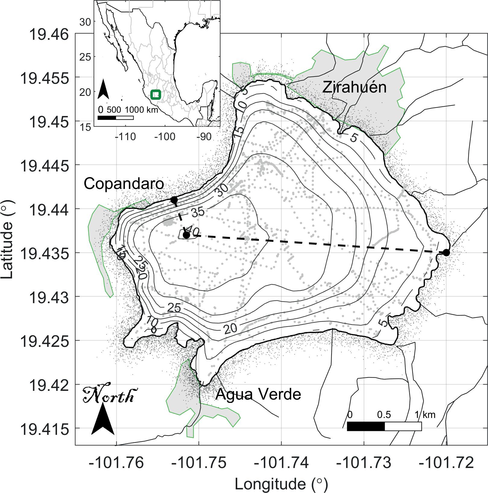
Figure 1. Location, bathymetric chart and bathymetric survey of Lake Zirahuen. The black isolines are marked every 5 m. The gray dots represent the route of the surveys. The shaded areas correspond to the local communities at the rim of the lake. The black dashed line shows the transect to estimate the slopes of the lake. The black lines reaching the lake correspond to the discharge of runoff water. The green rectangle of the inset shows the location of the lake in Mexico.
2.1In-situ Observations
2.1.1Morphology
The actual bathymetry and shoreline data required for the model configuration were obtained from measurements made on several expeditions during February, May and November 2018 (Gasca-Ortiz et al., 2020). To make the bathymetry, a Lowrance Elite Fishing System echosounder with a Global Positioning System (GPS) integrated (Lowrance FS, Navico; Tusla, OK, USA) was used. The datum used by this system was the WGS 84, and although the lake may vary its depth according to the season of the year (mainly during dry season), the survey taken for these campaigns can be considered to have the same level of reference according to the elevation (~2076±1 meters above sea level) registered by the GPS. A bilinear interpolation was applied to the measurements to obtain the bathymetry chart.
It is observed that the greater depths were found towards the western part of the lake,
which reaches 40 m, meanwhile, the shallower portion of the lake is located on the eastern
side (Figure 1). Note that besides the lake being deep,
it also has very steep side walls that make it more complex (Thorpe, 2013). In this case, the slopes of the lake range from ~0.08
(
2.1.2Meteorological variables
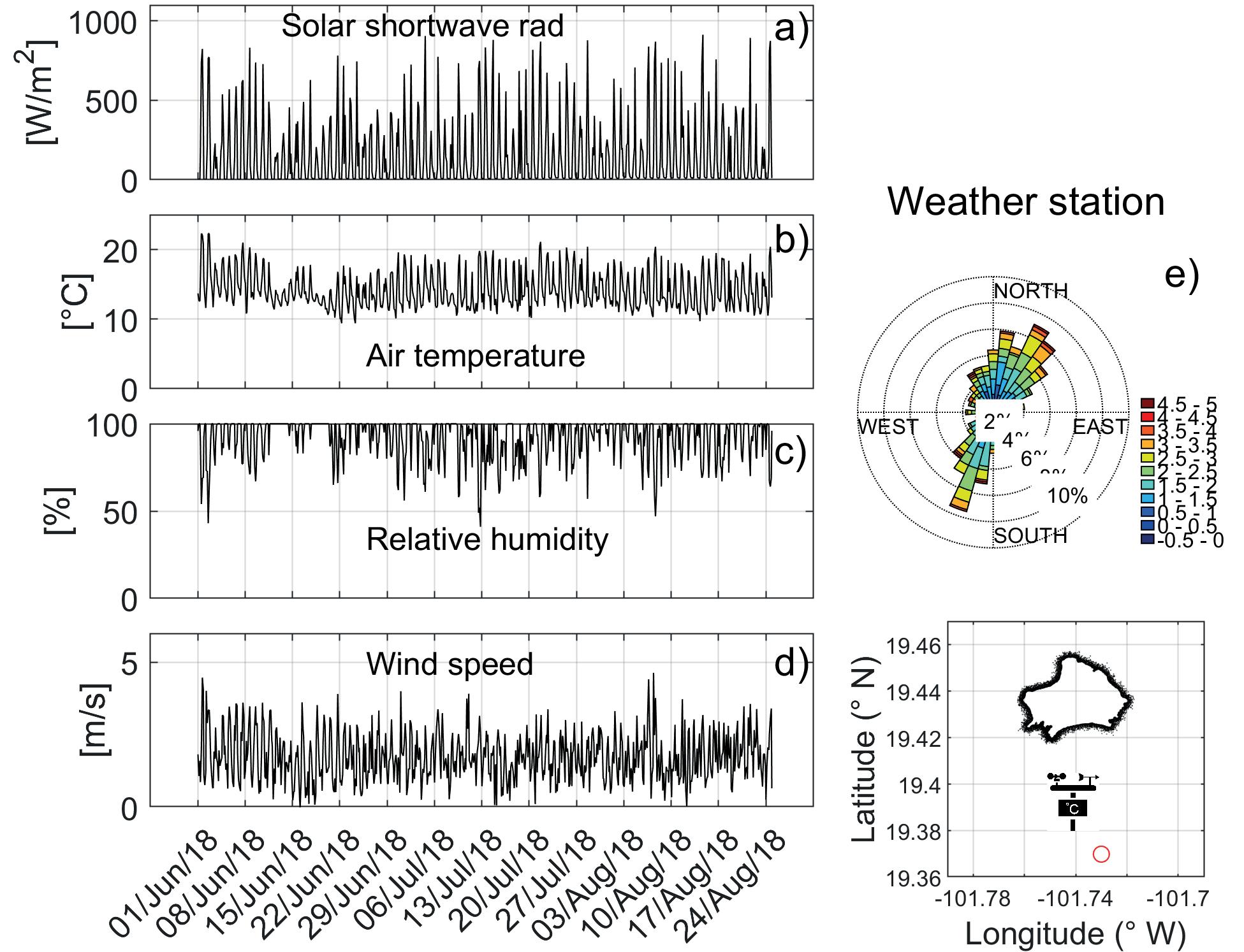
The surface forcings were retrieved from a meteorological station located at the southern side of the lake at approximately 10 km from it, with a HOBO micro station H21-002 (Onset Computer Corporation, Bourne, MA, USA) along with a Davis anemometer (Davis Instruments, Hayward, CA, USA). For the atmospheric variables, only four months were recorded from June to August 2018 (Figure 2). These data sets will be considered for the summer period.
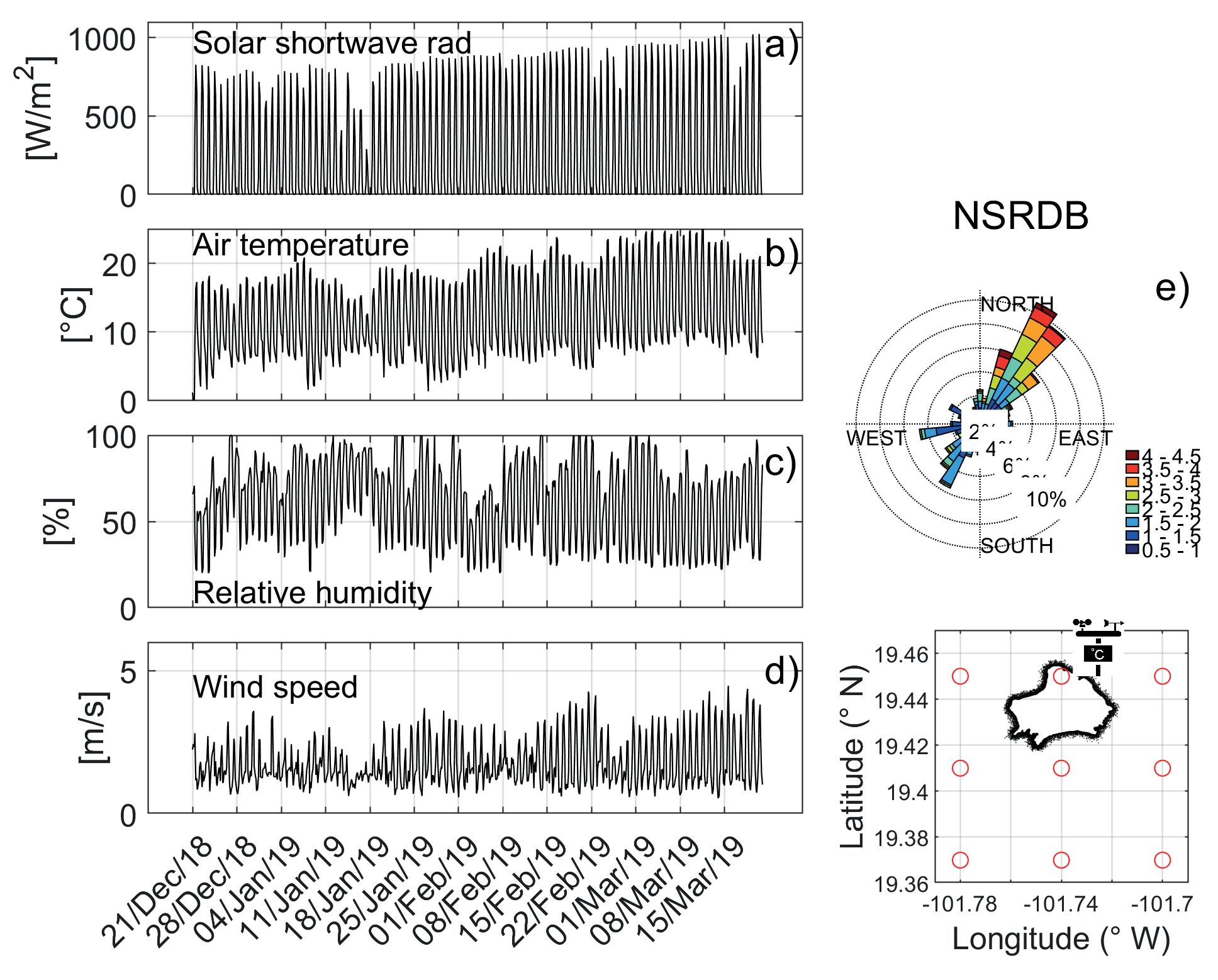
With respect to the winter season, data from the National Solar Radiation Database (NSRDB) of the National Renewable Energy Laboratory (NREL) were used from December 2018 to March 2019 (Sengupta et al., 2018). These data comes from a satellite-based model of meteorological information with a spatial resolution of 4 km and a temporal resolution of an hour, (Figure 3). These data can be downloaded from https://nsrdb.nrel.gov/. The nearest point in the lake was used to force the numerical model (see map in Figure 3).
2.1.3Stratification of the lake
The temperature field of Lake Zirahuén was measured also during those expeditions of February, May and November 2018, with a Conductivity, Temperature, and Depth-probe (CTD-probe XR-620, from RBR Ltd.; Ottawa, ON Canada) with a sampling rate of 1 Hz, which was lowered manually from the boat. The typical vertical profile for each season is shown in Figure 4. A simple linear interpolation procedure was applied to the measurements to fit the layers used in the numerical model (see next subsection).
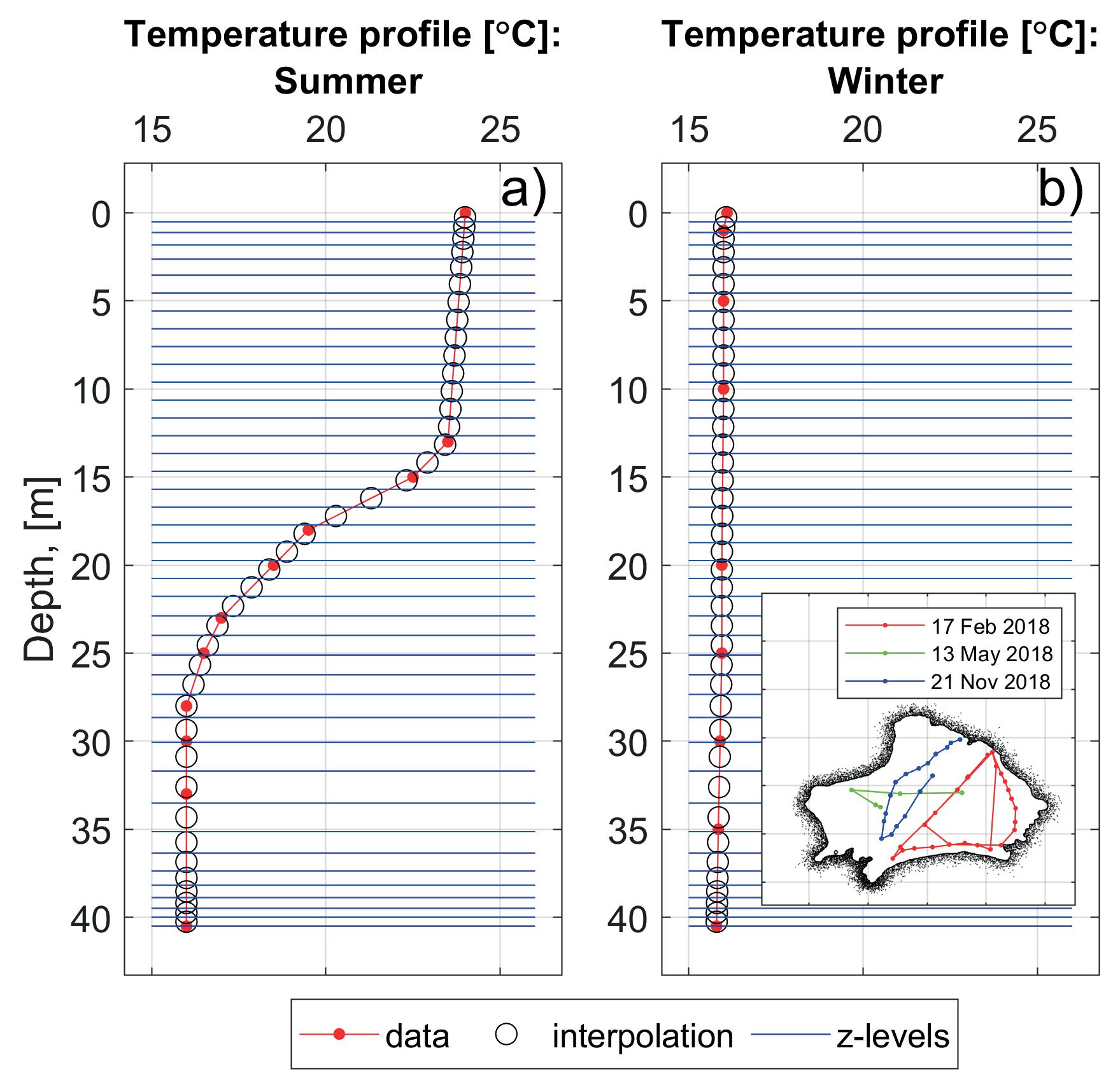
Figure 4. Temperature profile for (a) summer and (b) winter. Red dots are the measurements, in black circles the interpolation applied, and the blue lines represent the layers used in the numerical model. The inset map shows the survey of the CTD taken during the corresponding dates, red in February, green in May and blue during November.
2.1.4Velocity field of the lake
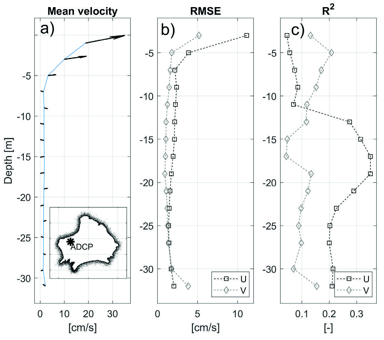
The horizontal velocities were measured from an anchor arranged with an Acoustic Doppler Current Profiler (ADCP, AquaPro 400 kHz; Nortek USA Inc., Boston, MA, USA) located at the maximum depth of the lake (Figure 5). It measured the vertical profile of three current speed components at a sampling rate of 5 min and a spatial discretization of 1 m from the near bottom to the surface. These measurements constitute a time series from July to August 2018.
To validate the numerical model (see next subsection), the following metrics were considered
for verification: the root mean square error
2.2Numerical Model
The numerical model Delft3D was used to calculate the tridimensional velocity field along with the thermal structure of Lake Zirahuén using the FLOW-module, meanwhile the Lagrangian particle trajectories were computed using the PART-module (Deltares, 2024b, 2024a; Lesser et al., 2004). The Delft3D model solves completely the flow hydrodynamics using the Navier-Stokes equations, the equation of state, and an equation of transport for the temperature, in shallow water systems. The governing equations are expressed in orthogonal curvilinear coordinates. The spatial discretization for both the equations and the physical domain was obtained by a finite difference scheme. This model was used particularly by Gasca-Ortiz et al., (2020) to study the circulation and thermal behavior of the lake. The time series of meteorological data necessary to force the model was obtained from two main sources: a nearby meteorological weather station and the NSRDB satellite-based model (see Figures 2 and 3). These forcings describe the temporal evolution of the most important variables that state the thermodynamic regime of the lake for each indicated season.
The PART-module of the Delft3D-suite model was configured to run offline from the FLOW-module. The numerical parameters to be adjusted for the passive particle tracking experiments were: the number of released particles, the initial release points and the horizontal parameters of dispersion (see next subsection), (Deltares, 2024a).
2.3Numerical scenarios
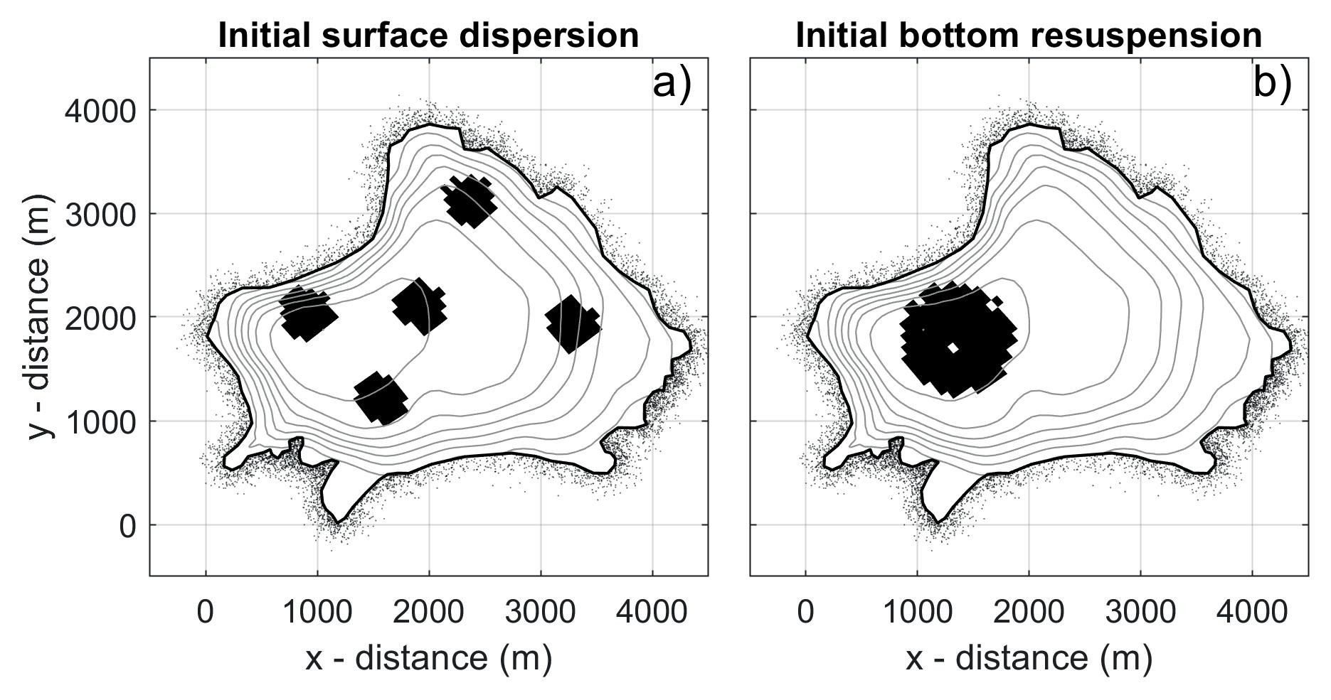
The numerical simulation was carried out during summer with a stratification state and during winter with an isothermal state (see Figure 4 for the thermal structure of the lake). Also to address the possible connectivity in the lake, two hypothetical scenarios were considered to describe the dispersive processes at different time scales within the study seasons. The first one represents a generic scenario where the initial release was chosen on the lake's surface, spanning its four quadrants and the central region (Figure 6a). This will allow the verification of the exchange between the different areas of the lake and between its main layers, with the particular objective of analyzing the discharge of wastewater runoff from the local settlement at the northwest region of the lake. This could represent the transport of contaminants or dissolved material by anthropogenic considerations (see Figure 1). The other hypothetical scenario will represent a process of resuspension from the bottom of the lake at the deeper region (Figure 6b), which, under certain thermodynamic and biological conditions, this case will represent a natural or typical occurrence in which an upwelling process may promote an algal bloom event.
2.4Numerical configuration
2.4.1Hydrodynamic model
The spatial domain that represents the entire lake was discretized with a high horizontal
resolution of ∆x, ∆y of ~70 m in a 61×36 grid size. Because the lake is considered deep and
steep-sided, in the vertical coordinate 40 zeta-layers were used with a resolution
The period of simulation was 90 days, of which 10 days were enough to warm up the model.
Actually, a day was enough to stabilize the thermal structure, while the velocity currents
take around five days to reduce the noisy signals. The time step allowable by the Courant
criterion was 15s. The wind stress was parameterized based on the wind drag coefficient
2.4.2Dispersion model
Even though the hydrodynamic simulation of the FLOW-module lasted for 90 days, the PART-module lasted only 30 days, since this was the time allowed due to the size of the lake, afterwards the connectivity in the lake was nearly homogeneous.
The PART-module also requires some numerical parameters to be adjusted for the passive particle tracking experiments: the number of released particles, the initial release points, among other parameters such as decay rates, vertical velocity, etc (Deltares, 2024a). The number of released particles during each hypothetical scenario from the stated location of Figure 6, was 100,000 particles. One aspect to note of the experiments performed in this study is that during the 30 days that each one lasted, the particles were released continuously, without any decay rates or an extra vertical velocity.
2.5Lagrangian dispersion
Each numerical particle will represent a fluid element with a certain duration and release position in the study area. From this Lagrangian point of view, the position of the n-th particle in the model is followed by its local coordinates at each instant t, as:
Here
where
with
The advective part of Eq. 1 was solved analytically based on a linear interpolation of the velocity, in which first, the spatial component was bilinear interpolated according to the actual position of the particle, considering the borders of the computational grid, and then the temporal integral was solved with respect to two consecutive velocity outputs (Deltares, 2024a).
2.5.1Lagrangian Probability density functions (LPDFs)
The hydrodynamic connectivity considered in this study will be defined as the probability
that some parcels of water are transported from one site to another, given a time period τ
(Li et al., 2014; Mitarai et al., 2009). By considering this advective time scale τ, the discrete
representation of the Lagrangian Probability density function (LPDF),
where x is the position, N is the total number of particles released in the domain,
The analysis of connectivity in the vertical direction is proposed in the same way.
2.6Drifting buoys and the horizontal dispersion coefficient
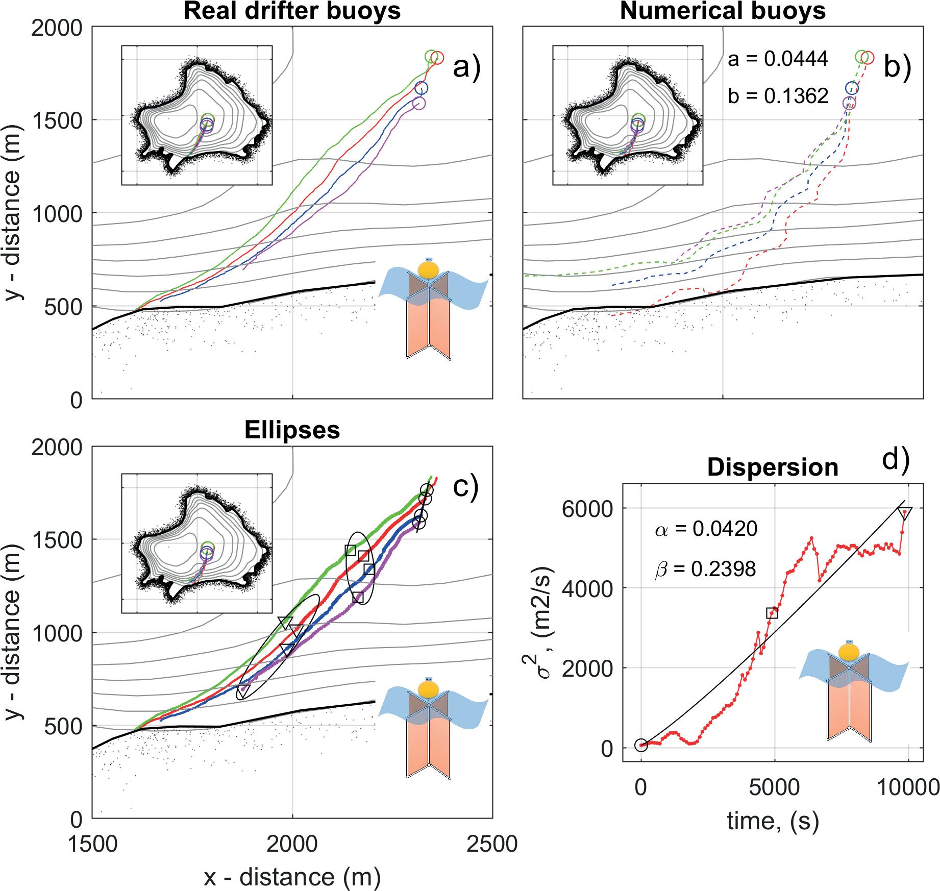
Data from a horizontal dispersion experiment of four drifting buoys in Lake Zirahuén were used to calibrate the PART-module (Eq. 3). Figure 7a shows the geographical location of the buoys released and their trajectories. The four surface buoys were deployed on September 28, 2022, from ~8:26 am to 1:37 pm; specifically, the red-buoy was deployed from 8:26 am to 1:31 pm; the green-buoy from 8:47 am to 1:37 pm; the blue-buoy from 9:05 am to 1:14 pm and the magenta-buoy from 9:20 am to 12:04 pm.
Those real trajectories were used to calibrate the parameters of the horizontal dispersion coefficients, a and b, of eq (3), based on a non-linear least square fitting calibration procedure that adjusts the best value for the model configuration (Figure 7b). The non-linear least square fitting procedure consists of determining α and β such that the following equation:
will be satisfied (Emery & Thomson, 1997; Lawrence et al., 1995; Okubo,
1971; Peeters & Hofmann, 2015), see Figure 7d. Here,
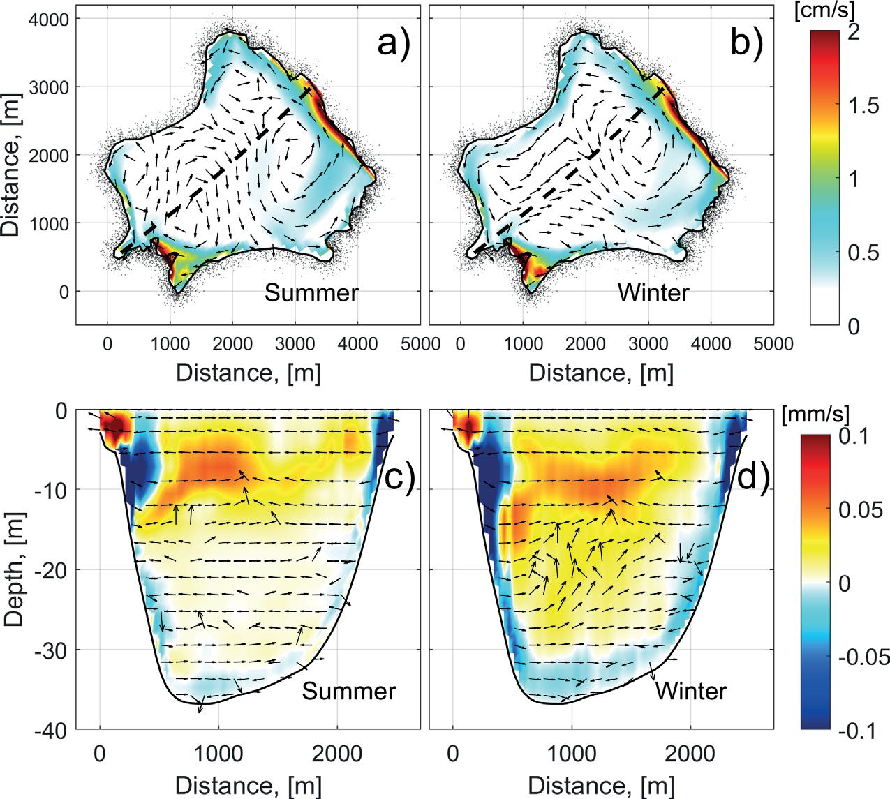
Figure 7. (a) Drifting buoys trajectories in Lake Zirahuén. The color circles show the initial point where the buoys were released, (b) the trajectories from the numerical model, (c) variability ellipses of real buoys, and (d) temporal distribution of the numerical ellipses enclosing the drifter ensemble.
3.Results
3.1Velocity validation
The average velocity profile of the ADCP is shown in Figure
5. It is observed that more intense dynamics are taking place at the surface layer with
velocities up to 30 cm/s, in accordance with what is expected in the first 5 m due to wind
stress and heat fluxes (Figure 5a). The rest of the layers
behave homogeneously, characterized by an average dynamic of relatively low intensity (<5
cm/s). In general, the model shows acceptable agreement with observations over all depths,
starting from 5 m to the bottom. The RMSE is considerably homogeneous and close to zero
(<1cm/s) below 5 m depth (Figure 5b). In the case of
3.2General Circulation
The numerical results are presented comparatively for mean values during the summer and winter periods, respectively, in Figure 8. It is observed that the hydrodynamics do not present higher intensity since the magnitudes of the estimated average velocities do not exceed 2 cm/s, something that is typical in this small lake (Gasca-Ortiz et al., 2020). However, the directions of the currents are more variable because they are subject to the stress of the wind and oscillate according to it. The horizontal movement is divided into two opposite centers of circulation: a cyclonic eddy to the northeast and an anticyclonic eddy to the southwest (Figure 8a, b). This characteristic pattern occurs in each period with minor differences in the position and extension of such eddies, for example, during summer, the structure of the circulation is nearly symmetrical with respect to the east-west orientation (Figure 8a), meanwhile in winter, the cyclonic eddy has greater extension, covering the large part of the northern side of the lake (Figure 8b). With slightly seasonal differences in extension, those structures generate more intense boundary currents that could transport debris and other substances along the coast.
The vertical component of the velocities in the lake is shown in Figure 8c, d through the cross-section in a north-south direction (see Figure 8a). Although the magnitudes of the vertical velocities are in the order of 0.1 mm/s, it is a very important variable due to the processes of vertical transfer and mass exchange of different tracers between the main layers of the lake.
On the contrary to the similarity with the horizontal circulation, the vertical structure presents a very different arrangement for each period studied; in particular, the summer stratification (Figure 8c) almost inhibited the vertical circulation, while in the winter season covers the entire water column (Figure 8d). In the latter season, it is verified that the vertical component of the flow has a higher magnitude and more variability. In this case, downwelling currents are generated close to the coastal area and flow along the ends of the lake towards the bottom because the action of the wind has a preferred northward and southward direction due to the valley-mountain breeze (See Figure 2 and 3 and Gasca-Ortiz et al., (2020)). This result indicates the probable occurrence of a persistent process of entrainment of water masses from the surface into the epilimnion and up to different depth levels of the metalimnion or even reaching the hypolimnion layer. Then, the vertical component of the velocity is predominant, and therefore, there is an intense vertical dynamic where circulation cells and vertical currents develop throughout the interior of the lake.
3.3Connectivity
3.3.1Verification of Lagrangian trajectories
Regarding the experiments of the drifting buoys (Figure 7a), these observed trajectories were used to estimate the virtual trajectories generated in the PART-module (Figure 7b), in order to obtain the adequate parameters, a and b, for eq (3). In this case, the methodology applied by Peeters & Hofmann, (2015) was used to determine the dispersion coefficients based on variability ellipses computed from trajectories taken from 9:20 am and 12:04 pm (aprox. 3 hrs) (Figure 7c and d). As noted in Figure 7a and 7b, the total displacement agrees within the real and virtual particles generated in the numerical model; that is, the modelled velocity field seems to be adequate, at least for the space-time scales considered in this study. Then, according to these results, the numerical solutions obtained from the Lagrangian trajectories will be considered as an acceptable and adequate approximation to model the connectivity based on the LPDFs.
The numerical results previously presented are the main components used to calculate the individual Lagrangian trajectories from which the connectivity is estimated, and hence the predominant dispersive patterns in each study period. In this sense, according to the scenarios considered in Figure 6, the LPDFs were calculated for the lake.
3.3.2Initial surface dispersion scenario
3.3.2.1Horizontal Connectivity
Note that the horizontal LPDF (relative number of particles per m²) was vertically integrated. In Figure 9, it is observed that during summer, there is a marked connectivity between all areas of the lake due to a greater dispersion in which nearly all the horizontal region is covered for τ > 15 days. These features are less accentuated in time scales τ < 15 days because the predominant wind direction is in the north-south direction, which tends to accumulate particles over the lake's northwest corner. In this west region of the lake, the connectivity patterns seem to align with the coast from time scales of τ = 1 day (Figure 9a) and holds approximately for τ = 3 days (Figure 9b).
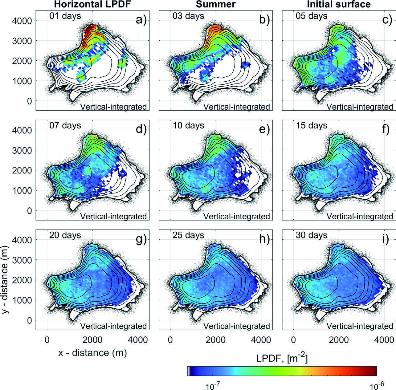
Figure 9. Horizontal connectivity of Lake Zirahuén during summer. LPDF for different time scales. (a) τ = 1 day, (b) τ = 3 days, (c) τ = 5 days, (d) τ = 7 days, (e) τ = 10 days, (f) τ = 15 days, (g) τ = 20 days, (h) τ = 25 days, and (i) τ = 30 days.
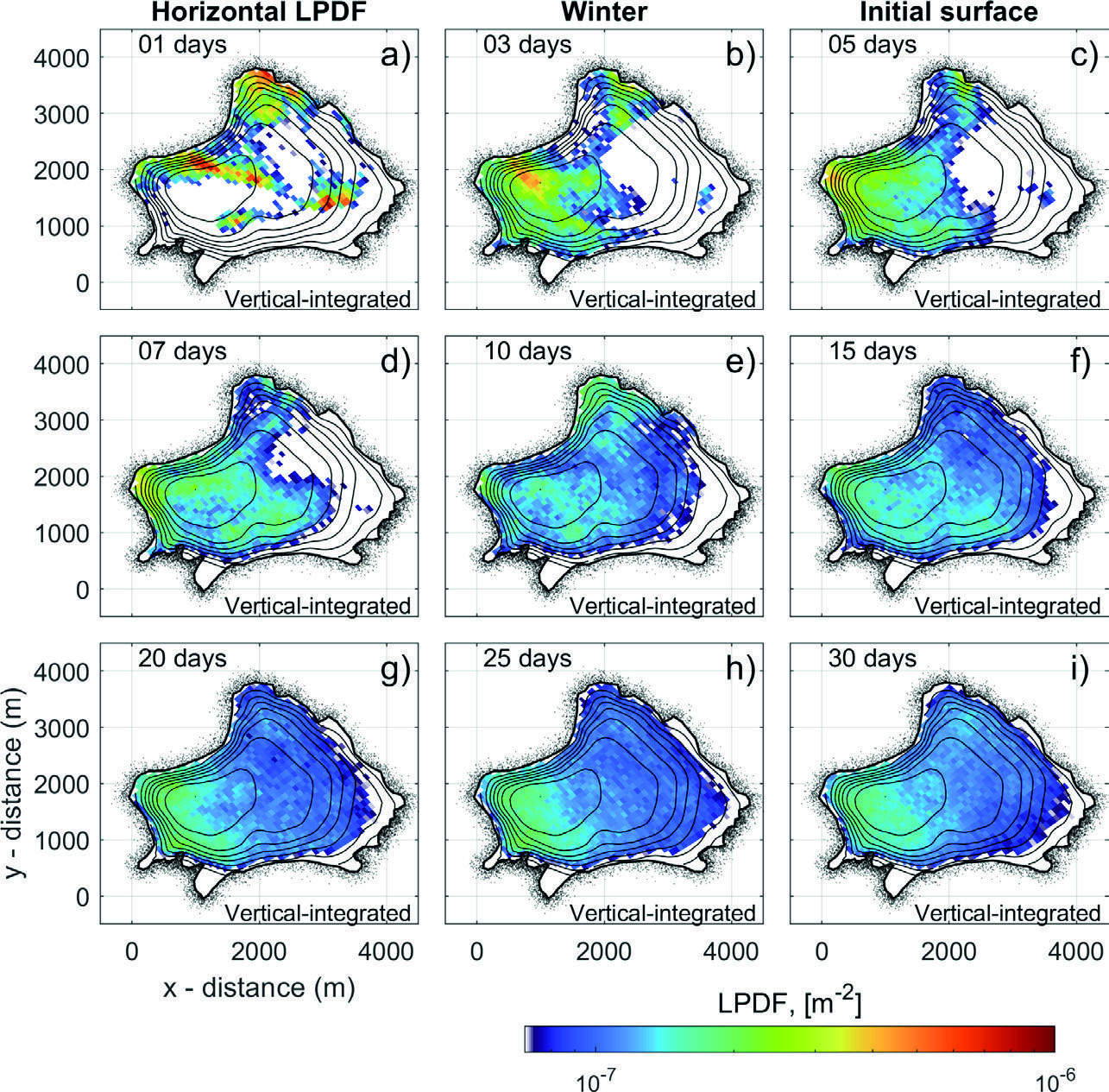
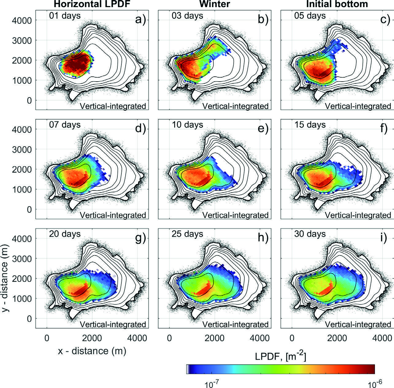
In winter, there is a marked difference in the connectivity for τ < 5 days (Figure 10) compared with the summer season. In this case, the accumulation of particles starts at the west coast of the lake at τ = 1 day (Figure 10a), but then they begin to aggregate at the southwest corner of the lake for 3 < τ < 7 days (Figure 10). Afterward, the connection of all areas is similar to the summer case, although the probability of reaching every place in summer is slightly less than in winter.
3.3.2.2Vertical Connectivity
The vertical component of connectivity is shown in Figures 11 and 12. Note that the vertical LPDF (relative number of particles per m) was horizontally integrated.
In summer, the particles concentrate mainly on the surface layer. For τ < 1 day, it shows a tendency to concentrate at the epilimnion (<5 m); meanwhile, for τ > 1 day and forward particles are in depths less than 10 m (Figure 11). This pattern is maintained for higher time scales, where considerable vertical displacements generally do not exceed 10 m, that is, they do not penetrate the top or the upper part of the metalimnion. Below that level, the probability is negligible due to the present stratification that constrains the vertical movements.
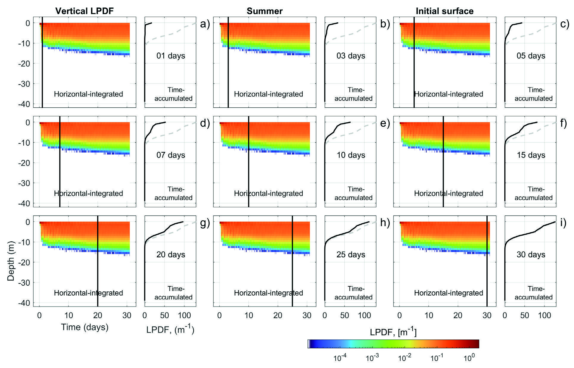
Figure 11. Vertical connectivity inside Lake Zirahuén during summer. The temporal evolution is the same as Figure 9. Each panel has two graphical representations: in the left is shown the temporal evolution of the vertical-LPDF with the black-line marking the current time. To the right is the time-accumulated vertical-LPDF marked with the continuous black line. The discontinuous gray-line corresponds to day 30.
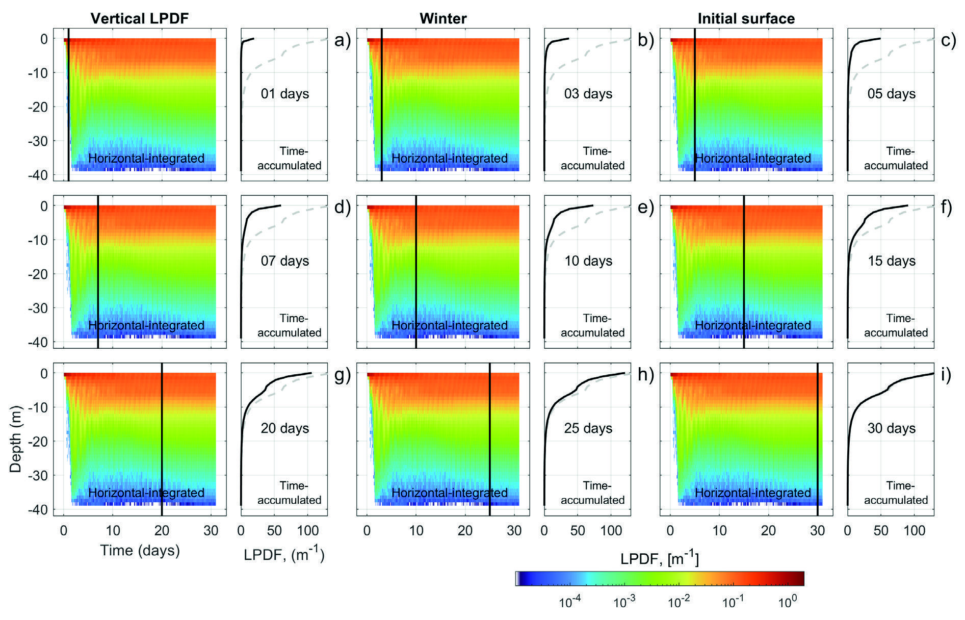
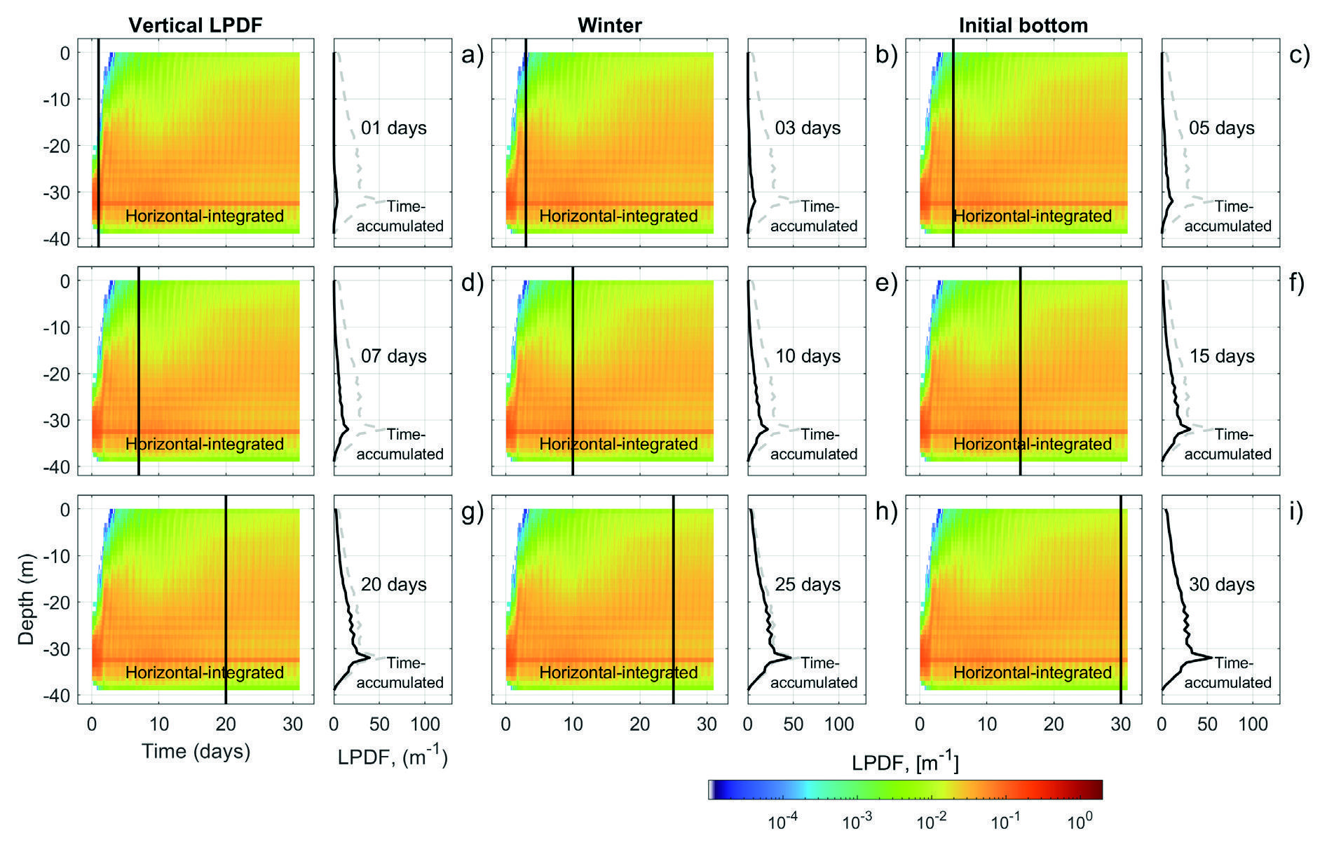
During winter, the vertical connectivity is totally different from the beginning, contrary to the horizontal dispersion (Figure 12). In this case the particles can spread to all depths rapidly. For example, between τ ~ 1 day and τ ~ 3 day, there are values of LPDFs reaching depths up to 20 m considering a threshold of 10-2 m-1. It is observed clearly that although most of the particles remain on the surface layer from 0 to 20 m deep, a few can travel to deeper layers.
3.3.3Connectivity on the initial bottom resuspension scenario
3.3.3.1Horizontal Connectivity
This scenario is related to the bottom layers, and it is proposed to estimate the vertical sediment uplift. It is observed that the dispersion of the horizontal displacement is very low for time scales of τ < 7 days, where the cloud of particles moves in the order of hundreds of meters in the summer case (Figure 13a to d), so larger time scales are required for dispersive processes to reach much of the horizontal dimensions of the lake. Then from τ > 10 days and forward, there is more dispersion, but it seems restricted to 30 m depth. According to these results, that distribution remains for times up to τ = 30 days. The results show that the dynamics of the lake's bottom are less intense compared to the surface connectivity, as can be seen in the main nucleus of particles that do not present the same dispersive features as the previous case, where the former move more slowly and concentrated around the initial position (Figure 13 and 14), not like the latter (see Figure 9 and 10).
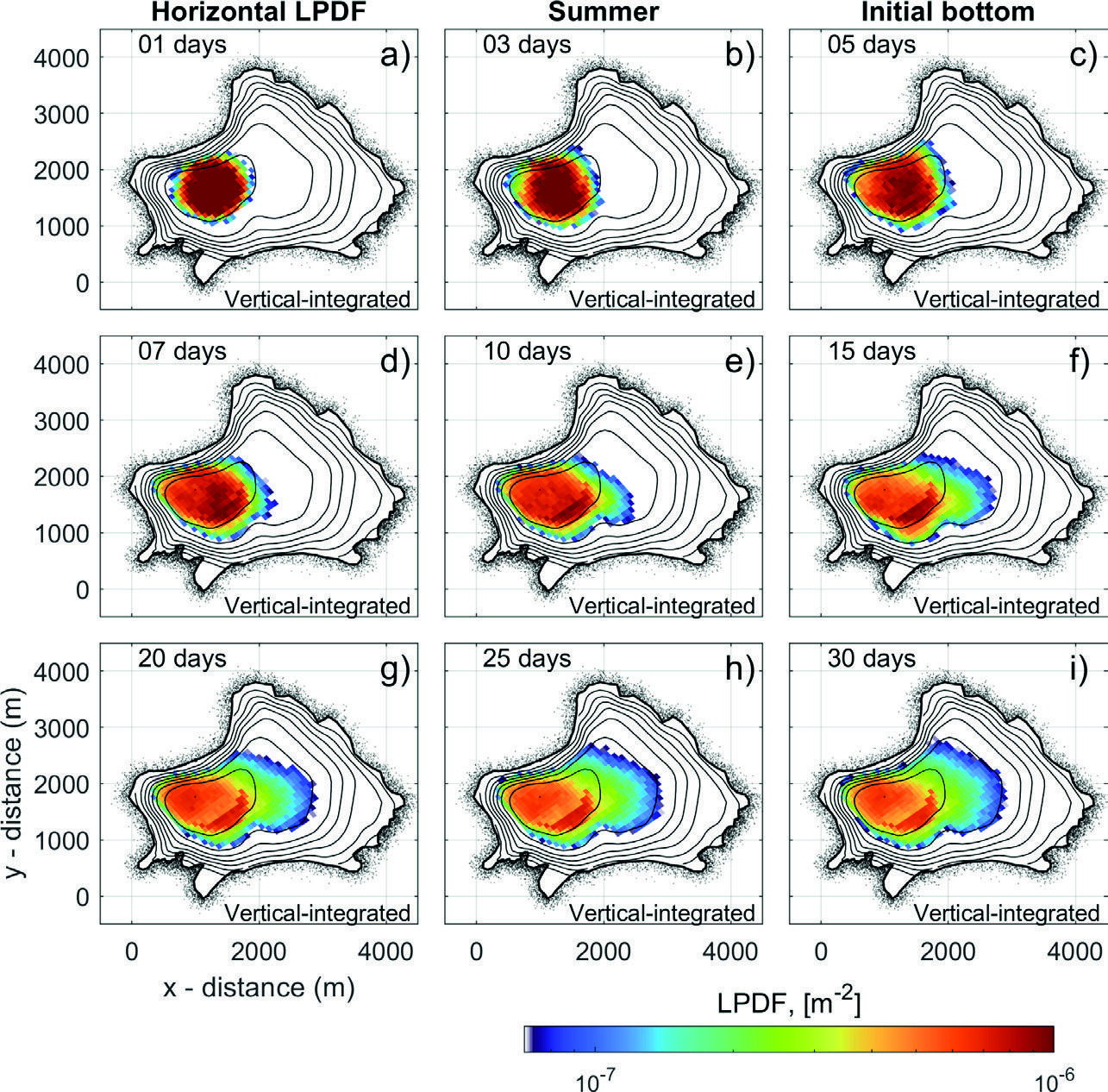
Figure 13. Horizontal connectivity from the bottom of Lake Zirahuén during summer. Same as Figure 9.
For the winter case, the dispersion of horizontal displacement shows more variability for time scales τ < 3 days, than the summer case (Figure 14). Then from τ > 5 days and forward, there is more dispersion not so constrained to the depth of 30 m but with a tendency to go to the sallower region of the lake on the east coast.
3.3.3.2Vertical Connectivity
In summer, the particles concentrate mainly on the bottom layers, below ~30 m depth (Figure 15). The time series evolution does not present any significant variability besides the onset before τ < 5 days, afterwards the particles tend to accumulate below the thermocline.
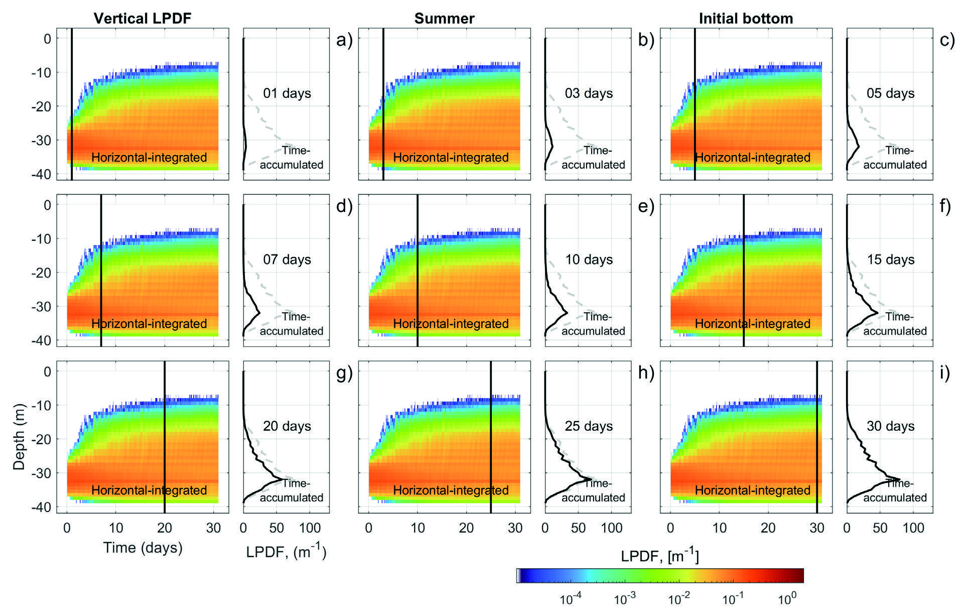
Figure 15. Vertical connectivity from the bottom inside Lake Zirahuén during summer. Same as Figure 11.
However, during winter (Figure 16), the particles are able to extend to all depths rapidly, and practically for τ = 3 days, the particles are in the total water column. There is a nucleus around 30 m where all particles aggregate, but not so marked as in summer period. It seems that the particles will be distributed homogeneously in the whole lake.
4.Discussion and conclusions
4.1General Circulation
From the numerical simulations in both seasons, it is deduced that Lake Zirahuén presents relatively low intensity and variable current dynamics largely conditioned by the action of the wind, which produces a certain periodicity in the orientation of the velocity field. The predominant hydrodynamic regime generates more intense currents along the north coast, which are highly likely to cause the dispersion and transport of waste material and other substances.
One of the main interests in this study was the estimation of the vertical connectivity, since this allows the exchange that occurs between layers, and therefore a way to analyze several processes like mixing, vertical transport, water entrainment, resuspension, among others. In this regard, the magnitudes of the vertical velocities are of the order of 0.1 mm/s but still can be significant for the vertical transfer of material inside the lake with very important consequences like mixing and exchange processes between the different layers. The numerical results show the presence of vertical currents throughout the water column, mainly in winter. The development of closed circulation cells and some areas of velocity gradients in winter are also evident, where the most intense currents descend along the rims of the lake from surface to bottom or intermediate layers. These processes are associated with the entrainment of water into the lake (Pieters et al., 2024), which can occur due to several effects: wind-induced mixing and thermal convection from the surface, currents that converge in frontal areas, and gravity currents that are generated along the bottom slope. These processes play an important role in the distribution and homogenization of the water mass within the lake.
4.2Connectivity
The connectivity model was directly associated with dispersion patterns, in which the surface connectivity, as expected, responds mainly to wind forcing, and therefore, patterns of rapid change are obtained, reaching horizontal distances greater than 1 km during τ = 1 day. On time scales greater than τ = 10 days, horizontal connectivity was nearly uniform across the entire lake, which would imply approximately an equal probability of particle transport to all subregions of the lake, regardless of the initial site of particle release. On the other hand, the horizontal dynamics on the bottom of the lake were much less intense. The main particle nuclei do not present the same dispersion as the surface dispersion and move more slowly, concentrating around the initial position for τ < 10 days.
4.2.1Discharge of wastewater runoff
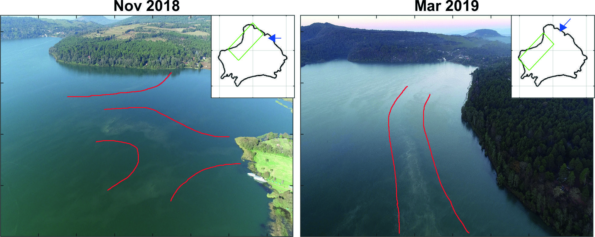
Both seasons and hypothetical cases were very different, allowing to relate these phenomena directly or indirectly with real problems linked to the deterioration of water quality and the ecology of the lake. As an example of this, is the transport of pollutants and their residence time inside the lake, as well as oxygen and other nutrients in the vertical and also algal bloom events. With this in mind, the surface scenario was also useful to reproduce the physical phenomena of discharge of wastewater runoff, which has a significant impact on the quality of the water and the ecology of the lake. In this sense, Figure 17 shows the evidence of real images taken by drone in November 2018 and March 2019, in which an elongated structure of suspended material running through the west coast of the lake is shown. This pattern was recurrently observed in the lake, and qualitatively, the simulated patterns have great similarity in terms of their shape and extension of the formation of elongated bands that developed nearly parallel to the northwest coast, extending for more than 2 km for time scales greater than 3 days (see Figure 9a).
4.2.2Algal Bloom
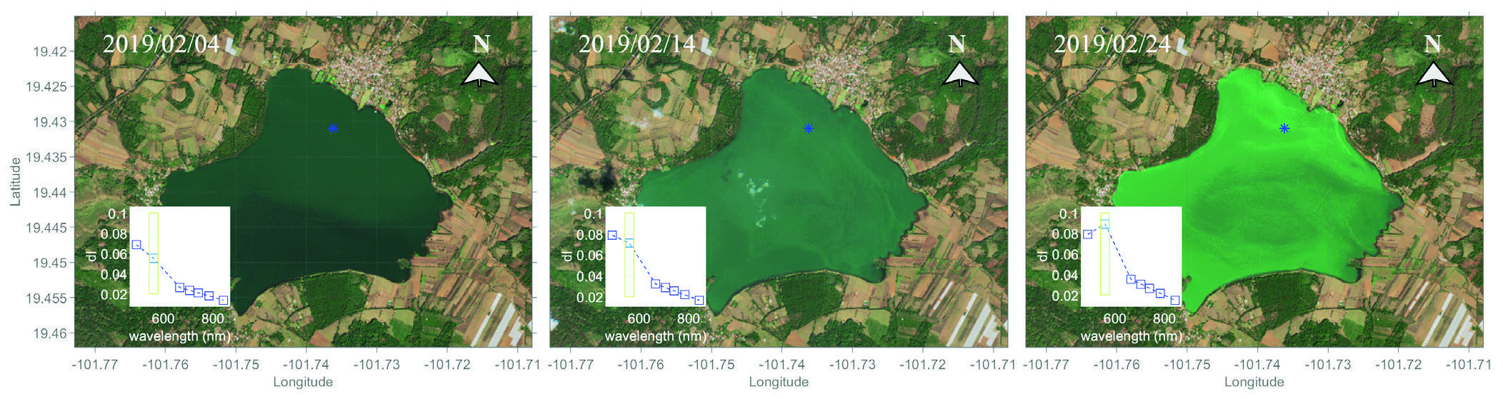
Also, it is worth mentioning that there have been some events of algal blooms registered in the lake that took place mainly during late winter. The physical processes involved in such events are related to the lifting of sediments, as the one simulated in the resuspension case. For example, during February 2019 (late winter), a color-base satellite evidence shows that there was an algal bloom event that precisely took place in the order of 10 days to make visible its effects (Figure 18), and although an algal bloom event is more complex, it is remarkable that the simple connectivity process of this study captures this essential behavior, so these results encourage the reliability and validity of the model, used at least in this sense, to show the movement distribution of the Lagrangian particles.
4.3Final Remarks
The connectivity model of the lake showed a satisfactory numerical solution based on Lagrangian motion, making it possible to apply it to specific relevant processes such as the discharge of wastewater runoff and those related with algal blooms. In this sense, the knowledge of the hydrodynamic circulation and connectivity processes in the lake can contribute to activities for the conservation and comprehensive management of the lake as a resource. Besides, this study can be applied in both the prediction of dispersive patterns and as a guide for evaluating potential areas exposed to polluting sources and other types of substances of suspended or dissolved matter. The above can be relevant for implementing regulatory standards to promote the sustainable development of the lake ecosystem in balance with the human activities involved. Furthermore, the methodology is fully extensible and easy to adapt to other regions.
Considering winter, this season seems to be a monotonous period where everything appears constant as the lake gets its isothermal state. Nevertheless, the physical phenomena that develop these processes can be intriguing; for instance, the baroclinic instabilities or the internal variability in general that are expected to develop in the transition from summer to winter or the re-stratification from winter to summer, this needs to be analyzed in more detail, but are is out of the scope of this study.
Finally, the evaluation of the predictive capacity of Lagrangian motion in the lake was established using a sophisticated and versatile numerical model. However, we know that more rigorous quantitative validation for the hydrodynamics is required. In this regard, it is worth noting that the hydrodynamical results present in this study come from the study of Gasca-Ortiz et al., (2020) in which the surface velocity was poorly reproduced, though, the thermal state of the lake was satisfactorily validated. But, as the actual structures observed from the drone images in this current study were reproduced in the model without any specific configuration, this encourages us to continue using the model, nonetheless, to keep working on improving its hydrodynamical validation in future studies.
5.Acknowledgements
The authors acknowledge the interesting and helpful comments by two anonymous reviewers. DAP acknowledges the grant of project number 55176 from which the drifting buoys were built. DOAG acknowledges a scholarship from CONAHCYT. TGO acknowledges the support of the CONAHCYT postdoctoral project.
6.Appendix
Following (Okubo, 1971), there is one definition to approximate the apparent diffusivity as:
based on a length scale
But also, the diffusivity can be approximated by
Then following Lawrence et al., (1995) and a simpler version of Peeters & Hofmann, (2015), it is found that
And
Which have the same form of eq. (3) with

