


 nueva página del texto (beta)
 Inglés (pdf)
 Artículo en XML
 Referencias del artículo
 Enviar artículo por email
 Citado por SciELO
  Similares en
SciELO
Similares en
SciELO 
 Permalink
1. Introduction
The ground gravity field maps are widely used for mineral resources exploration programs. The obtained images consist of anomalies with various intensities and wavelengths which are covered by the noises with various amplitudes in most cases. Therefore, to extract the details on the map and highlight the structures and shape of gravity anomaly sources with various intensities, the filtering technique has been used. There are various filters to enhance and estimate the causative body edges of the potential field. Regarding the nature of the data and the domain of changes in the intensity of anomalies existing in the images as well as the filtering objective, various types of filters have been used.
Today, one of the filters widely used for the interpretation of gravity field data is the local phase filter. The most important advantage of such filters is their flexibility, in a way that, with a slight change in the formula of a filter, and in fact, their normalization, new and yet more efficient filters can be produced. Local phase filters are obtained by combining the horizontal and vertical derivative of gravity data with different orders. such as the analytical signal method (Nabighian, 1972 & 1974), the tilt angle filter (Miller and Singh, 1994), the total horizontal derivative (Verduzco et al., 2004), theta map (Wijns et al., 2005), the directional tilt angle and the real part of the hyperbolic tangent function (Cooper, 2006), balanced profile curvature filter (Cooper, 2009), generalized derivative operator (Cooper and Cowan, 2011), normalized total horizontal derivative filters (Cooper, 2006; Ma and Li, 2012), and angle of deviation of the total horizontal gradient filter (Ferreira et al., 2011 & 2013).
Yuang et al. (2014) suggested three optimized methods to balance the large eigenvalues of the data in a way that these eigenvalues are located on the edge of the anomaly source. Eshaghzadeh and Kalanatari (2017) offered the use of the Canny edge detection algorithm for the analysis of the potential fields. Görgün and Albora (2017) used the directive filter method to analyze the gravity fled. Eshaghzadeh et al. (2018) use the balanced generalized horizontal derivative tilt angle filter to analyze the potential field data. Also, the wavelet analysis method has been used to detect the border of the mass of gravity anomaly source (Alp et al., 2011; Ehaghzadeh et al., 2019).
All the mentioned methods detect the subsurface causative mass border on the map and practically they give no idea of how deep the edges of underground structure are. Thus, it is needed to, besides this edge detection method, also use another qualitative-quantitative method so that a correct interpretation of the area under evaluation and expansion of the subsurface source can be provided. To do so, we have used a 2-D inversion method to detect the vertical borders of underground mass. Numerous inversion methods have been provided by various researchers such as Kriging (Shamsipour et al., 2012), inversion by gravity gradient tensor (Hou et al., 2015; Zhen-Long et al., 2019), conjugate gradient method (Tai-Han et al., 2017; Tian et al., 2018), the weighted method (Rezaie et al., 2016), Modular Feed-forward Neural Network (Eshaghzadeh and Hajian, 2018), PSO algorithm (Eshaghzadeh and Sahebari, 2020), and damped SVD and Marquardt inverse methods (Eshaghzadeh and Hajian, 2022).
Through the error and trial and the use of various inversion methods, we finally concluded that using a reweighting focusing inversion method of the gravity horizontal gradient data is suitable for the detection of the edge of the subsurface anomaly source mass. The efficiency of this method is evaluated using two subsurface synthetic models, and in the following, real gravity horizontal gradient data due to a Chromite mass will be analyzed.
2. Methodology
In the linear inversion method, the subsurface ground is divided into a network of equal-sized cubes (cells) with a constant density contrast (in two-dimensional mode, the ground is actually divided into equal-sized rectangles along the data collection profile). The density contrast inside each cell is the unknown parameter in the linear inverse problem. Figure 1 shows an example of two-dimensional subsurface ground divided into equal cubes.
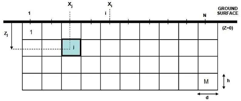
We need to calculate the kernel matrix (also known as the Jacobian matrix, the leading operator matrix, the sensitivity matrix, or the model matrix) for the gravity field. The kernel matrix is the calculation of the effects of gravity of each cube in Figure 1 (jth cube) in the point of calculation i. Therefore, considering Figure 1, in each point of calculation on the ground surface, NXM of gravity effect is computed.
Various formulas have been provided for the calculation of the gravity effect of the cube (in 3-D case) or rectangle (in 2-D case). The gravity effects of the rectangular block can be computed by following equation (Gerkense et al., 1989).
Where,
In the last equations, G is the gravitational constant,
Based on Figure 1, the equation of gravity linear inversion can be written as follows:
Where G is the Kernel matrix. The Kernel matrix represents the gravity effect of gridded subsurface inversion domain at all points of calculation on the ground surface without applying the density value of each cell (blocks of grid). In the gravity inversion, the objective is to determine the approximate response m (density contrast of each cell) using the known values of G and d (data vector). If the observed gravity anomalies are produced by M subsurface cells, the gravity anomaly in the ith point will be estimated as follows:
Where
In the gravity inversion, the Kernel matrix value quickly decreases with increasing depth. Therefore, the reconstructed model is focused near the surface, and it is needed to use a depth weighting function to neutralize the reduction in kernel sensitivity with depth (Li & Oldenburg, 1996; Pilkington, 1997).
2.1 Reweighting Focusing Inversion
The main objective of gravity inversion problems is to find a geologically acceptable density model based on the sensitivity matrix and the data measured at a level of noise. In the present study, we aimed to determine the density distribution that corresponds to the vertical borders of the mass subsurface structure, so our input data will be gravity horizontal gradient instead of gravity data. As mentioned, gravity inversion problems are usually ill-posed and the solutions can be non-unique or unstable. We can solve these problems by the minimization of Tikhonov parametric functional (Tikhonov & Arsenin, 1977):
Where
Where
To produce compact solutions, we select a stabilizer equal to the minimum support functional as follows (Portniaguine & Zhdanov, 1999):
Where
By placing the minimum norm stabilizing functional in Equation 6, we will have:
This problem is solved by the reweighting optimization (Mehanee et al., 1998). To calculate the various sensitivities of the data to the model's parameters, a diagonal weight matrix (
Where
In Equation 11,
Substituting the weighting matrix in Equation 9, and choosing
Where
and
Equation 12 is written as follows:
Equation 16 is similar to the classical minimum norm optimization problem whose solutions are based on the regularization theory (Tikhonov et al., 1977). The only prominent difference is the new progressive modeling operator, which is
Both expressions of the objective function (Equation 16) are 2-norm and thus, differentiable. The prevalent method to solve Equation 16 is using the least squares method. Then, Equation 16 is equal to:
Regarding the dominant relationships about gradient calculation, that is:
By computing the derivative of Equation 18 with respect to the model parameter
As a result, we will have:
The value of µ of the regularizing parameter is computed for each iteration as follows:
During the inversion, for each iteration, 2-norm error between the observed and computed gravity horizontal gradient data are estimated:
Where,
The 2-norm values of observed and computed gravity horizontal gradient difference in each iteration be less than the predetermined value, i.e.,
The 2-norm values of observed and computed gravity horizontal gradient difference in one iteration be higher than the previous iteration, i.e.,
The number of considered iterations for the inversion process be completed.
The modeling algorithm by the reweighting focusing inversion method is represented in Table 1.
Table 1. Reweighting focusing Inversion algorithm
|
Inputs: |
|
|
Stage 1: |
place
|
|
Stage 2: |
calculate
|
|
Stage 3: |
Calculate
|
|
Stage 4: |
Calculate
|
|
Stage 5: |
Calculate
|
|
Step 6: |
Apply density limits in a way that:
|
|
Stage 7: |
Place
|
|
Step 8: |
Check the stop criteria, if satisfied, stop the process, otherwise, go to step 3. |
|
Output: |
|
3. Analysis of Gravity Horizontal Gradient Data for Synthetic Models
In this section, two synthetic models are considered, and the computed gravity horizontal gradient data for these models will be analyzed using the reweighting focusing inversion method:
3.1 Synthetic Model No.1
Figure 2(a) represents the measured gravity field in 15 points on a gridded underground which has been divided into 150 cells as 9 of them have a density contrast of
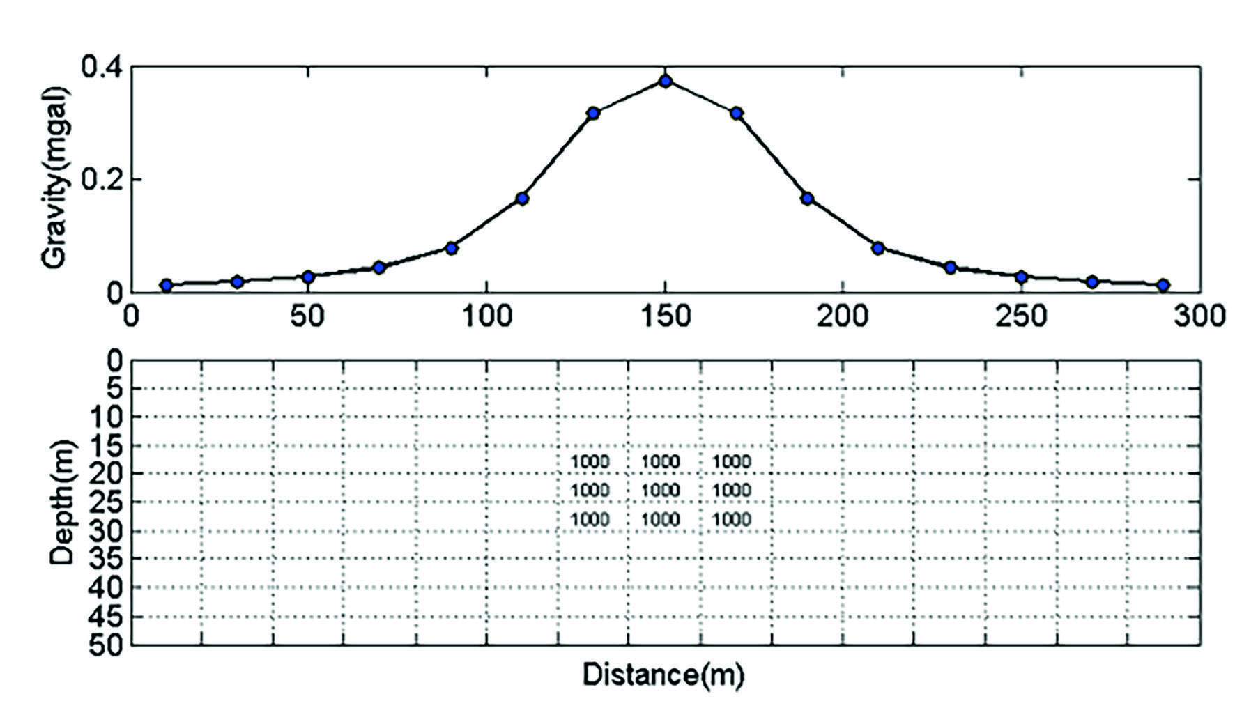
Figure 2. a) Alternations curve of the gravity field due to b) supposed subsurface model with a density distribution of 1000 kg/m3.
The value of the considered initial error between the computed gravity gradient and the inverted gravity gradient, as one of the stopping criteria for iterations in the inversion process, is equal to
The changes in the gravity horizontal gradient field of the synthetic model has been shown by the red curve in Figure 3(a). The subsurface density distributions resulted of the inversion with a different sign have been taken place on the vertical borders of the anomaly source (Figure 3(b)). The gravity horizontal gradient field obtained from the inversion is depicted in Figure 3(a) by the circle symbols and blue dashed lines.
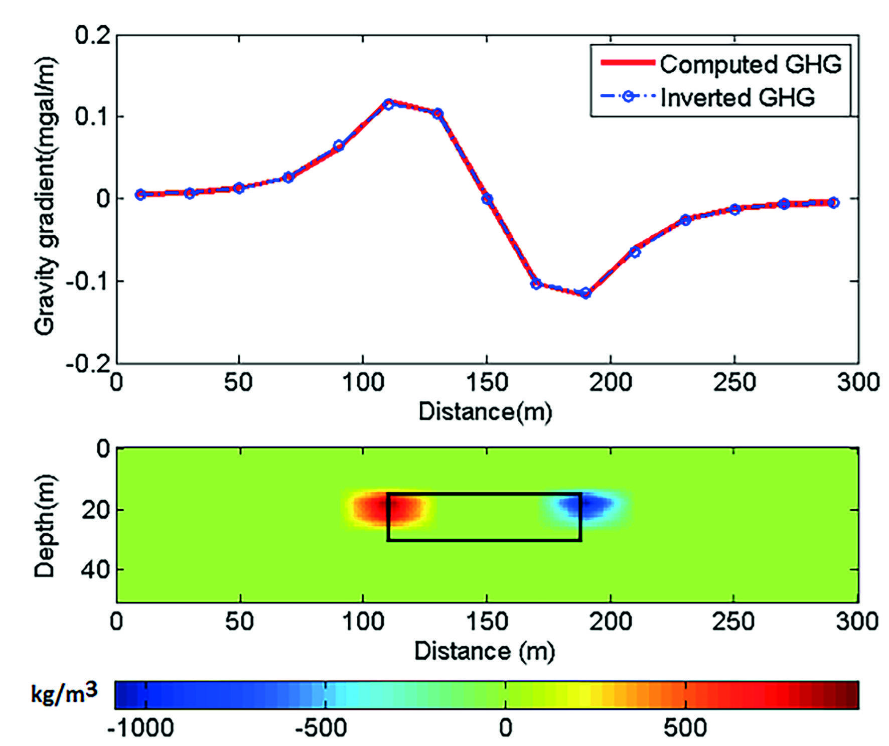
Figure 3. a) the computed gravity horizontal gradient and the horizontal gradient data obtained from the inversion according to b) Subsurface density distribution obtained from the inversion for the synthetic model No.1
As seen in Figure 3(b), the maximum and minimum values of gravity horizontal gradient are located on the vertical borders of the anomaly source mass, and the positive and negative density distributions corresponding to these values have clearly detected the depth of vertical borders. The gravity gradient is commonly used for edge detection. Although these density distributions could not estimate the depth expansion of the border clearly, they are able to detect the depth of the top surface of the anomaly body.
As seen in Figure 4, the 2-norm error value between the computed gravity gradient and the gravity horizontal gradient data obtained from the inversion reduces drastically in the 11th iteration and reaches to 0.0036mGal/m in the 12th iteration. This value is lower than the initial assumed error value and as a result, the inversion process was stopped.
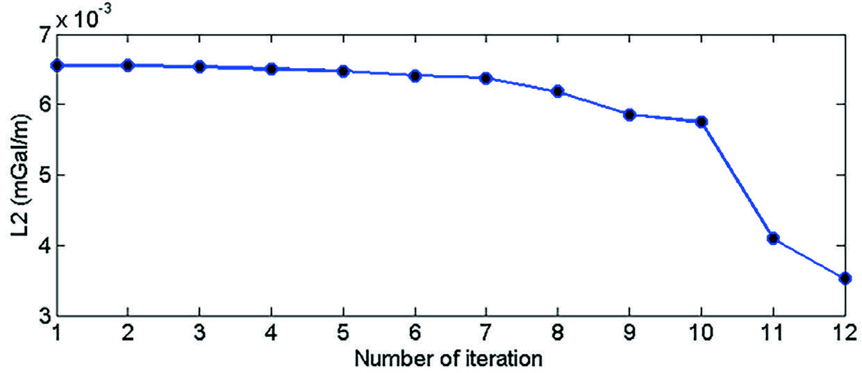
Figure 4. changes in the 2-norm errors between the computed gravity horizontal gradient and obtained ones from the inversion in each iteration for the synthetic model No. 1.
To examine the efficiency of the reweighting focusing inversion method with noise, 20% random noise is added to the theoretical gravity horizontal gradient field in Figure 2(a), based on the following equation:
The value of the considered initial error between the computed gravity horizontal gradient and the inverted ones, as one of the stopping criteria for iteration in the inversion process, is equal to
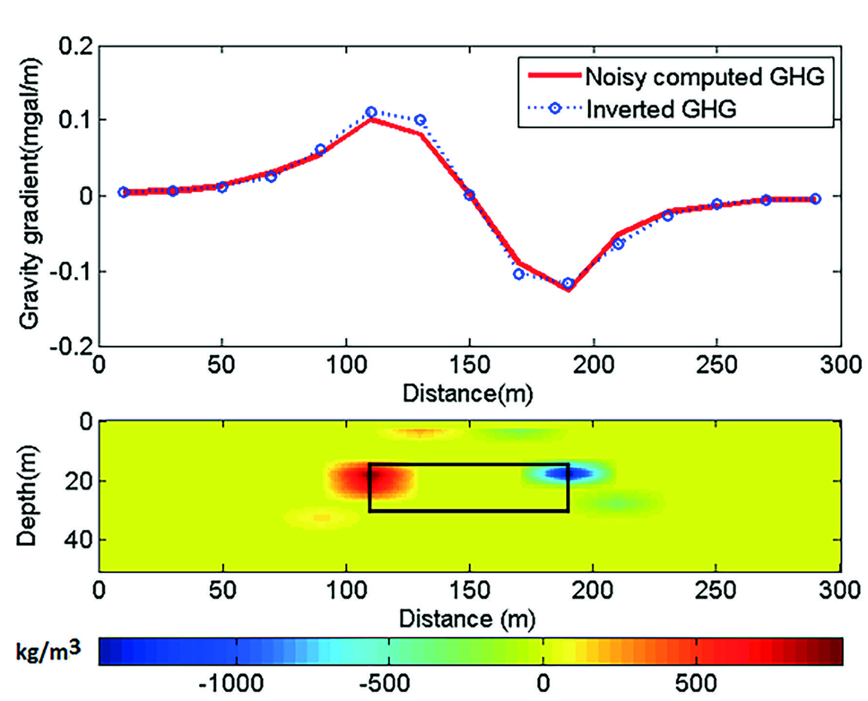
Figure 5. Noise corrupted synthetic gravity horizontal gradient and inverted gravity horizontal gradient due to b) recovered subsurface density distribution for the model No.1.
As seen in Figure 5(b), the maximum and minimum values of gravity horizontal gradient are located on the vertical borders of the anomaly source mass, and the positive and negative density distributions corresponding to these values have partially detected the depth of vertical borders.
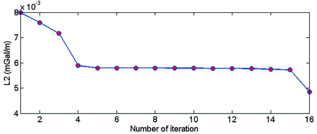
As seen in the last figure, due to the presence of the noise, several small density distributions with low amplitude have been also detected after inversion. Also, the positive density distribution has detected the depth expansion of the source vertical border better than the negative density distribution. As shown in Figure 6, the value of 2-norm error between the computed gravity horizontal gradient and inverted gravity horizontal gradient data shows a sharp decrease in the 16th iteration and reaches 0.0049 mGal/m, which is lower than the initial assumed error value, and as a result, the inversion was stopped in the 16th iteration.
3.2 Synthetic Model No.2
Figure 7(a) represents the estimated gravity field in 20 points on a gridded subsurface that is discretized into
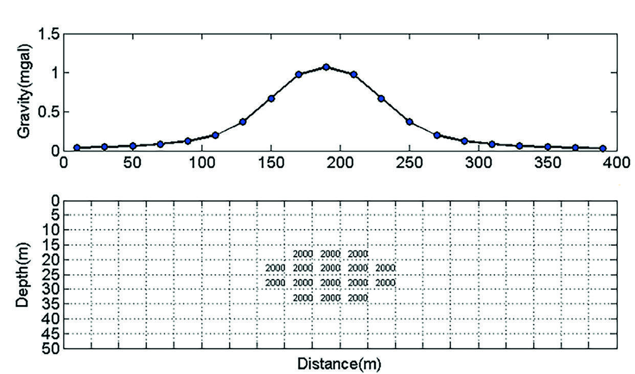
Figure 7. a) Alternations curve of the gravity field due to b) supposed subsurface model with a density distribution of 2000 kg/m3 (synthetic subsurface model No.2).
The value of the defined initial error between the computed gravity horizontal gradient and the inverted ones, as one of the stopping criteria for iteration in the inversion process, is equal to 0.04 mGal/m, and
The changes in the gravity horizontal gradient field of the synthetic model No.2 is shown by the red curve in Figure 8(a). Since the vertical border of the anomaly source is stepped, as seen in Figure 8(b), the maximum and minimum values of gravity horizontal gradient have almost conformity to the middle of the stepped border of the anomaly source mass. Nonetheless, the subsurface density distributions resulted from the inversion, where they have the different sign, have been located on the farther vertical borders of the anomaly causative mass and have been approximately detected their depth expansions (Figure 8(b)). Therefore, using the maximum and minimum values of gravity gradient as an edge detector of the anomaly source can include errors. The inverted gravity horizontal gradient data is shown in Figure 8(a) by the circle symbols and blue dashed lines.
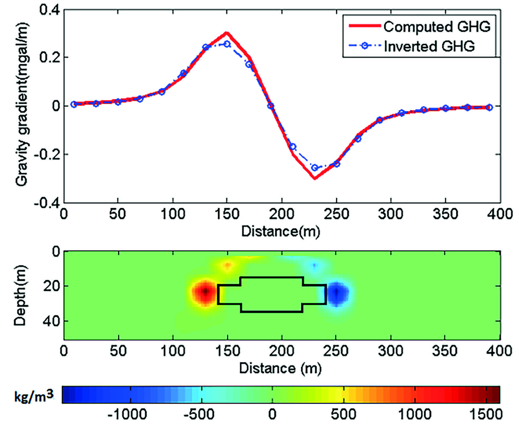
Figure 8. a) computed gravity horizontal gradient and the inverted gravity horizontal gradient due to b) recovered subsurface density distribution for model No.2
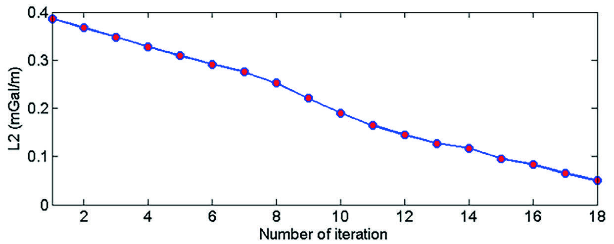
As shown in Figure 9, the value of error between the computed gravity horizontal gradient and the inverted ones is 0.0357 mGal/m in the 17th iteration, which is lower than the initial assumed error value, and as a result, the inversion was stopped in this iteration.
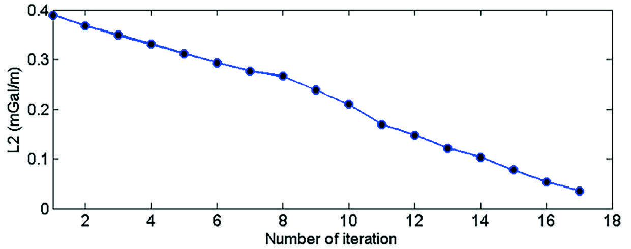
Figure 9. Alterations in the 2-norm errors between estimated gravity horizontal gradient and inverted gravity horizontal gradient in each iteration for the synthetic model No.2.
We have studied the proficiency of the reweighting focusing inversion method by adding 20% random noise to the theoretical gravity horizontal gradient data in Figure 7(a), based on Equation 27.
Figure 10(a) shows the gravity horizontal gradient field of the synthetic model No.2 by the red curve as is noise corrupted. The predefined error value was set as 0.06 mGal/m and
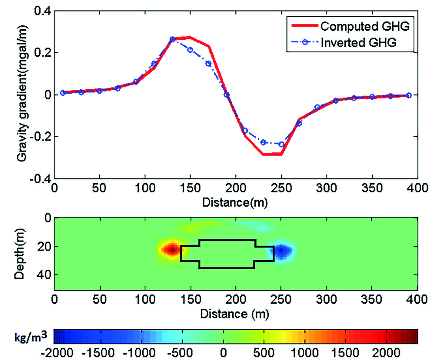
Figure 10. Noise corrupted synthetic gravity horizontal gradient and inverted gravity horizontal gradient due to b) recovered subsurface density distribution for model No.2.
As seen in the figure 10(b), due to the presence of the noise, several small density distributions with low amplitude in the underground sub-space have been detected.
As shown in Figure 11, the value of 2-norm error between the computed gravity gradient and the inverted horizontal gradient is 0.0506 mGal/m in the 18th iteration, which is lower than the initial assumed error value, and as a result, the inversion was stopped in this iteration.
4. Sabzevar Chromite
In this chapter, we will get familiar with the location and geological structure of the area under investigation in Sabzevar, and then, we will analyze the gravity horizontal gradient data due to a subsurface Chromite mass.
4.1 Location and Geology of the Studied Zone
The study area is located in the North 40m zone of UTM coordinates between the longitudes of 607000 to 607120 meters in the west-east direction and the latitudes of 4012200 and 4012300 meters in the south-north direction, between the cities of Sabzevar and Neishabur, which includes an area of about
In fact, the Sabzevar region is a part of the Ophiolitic region that extends from the east to the south of the country. The structural form of the study area is undoubtedly influenced by faults such as Darouneh and Taknar. The construction direction of this area follows the Darouneh fault direction.
The Sabzevar area contains a large number of chromite masses in the form of strings and large and small lenses. The igneous masses of this area are stretched in an almost east-west direction and are primarily composed of alkaline rocks. Chromite masses are spread irregularly but with a certain concentration in these rocks. The amount of their alloy is very variable. Baroz et al. (1984) attribute the age of the Ophiolitic complexes to the Upper Cretaceous (Koniasian).
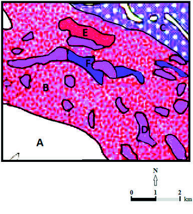
In the study area, the limited rock outcrops include ultrabasic igneous rocks that are mostly transformed into serpentine and minerals such as talc and vermiculite (Aghajani, 2013). Figure 12 shows the geological map of the area under study.
4.2 Gravity Field of the Study Area
Figure 13 shows the Bouguer gravity field of the study area in Sabzevar. As can be seen in figure 13, the gravity field has been measured along 6 profiles in the north-south direction and at 56 stations with an approximate distance of ten meters (black circles in Figure 13. Bouguer gravity field include the regional and local anomalies and by processing the Bouguer gravity field data can detect the positive and negative local anomalies.
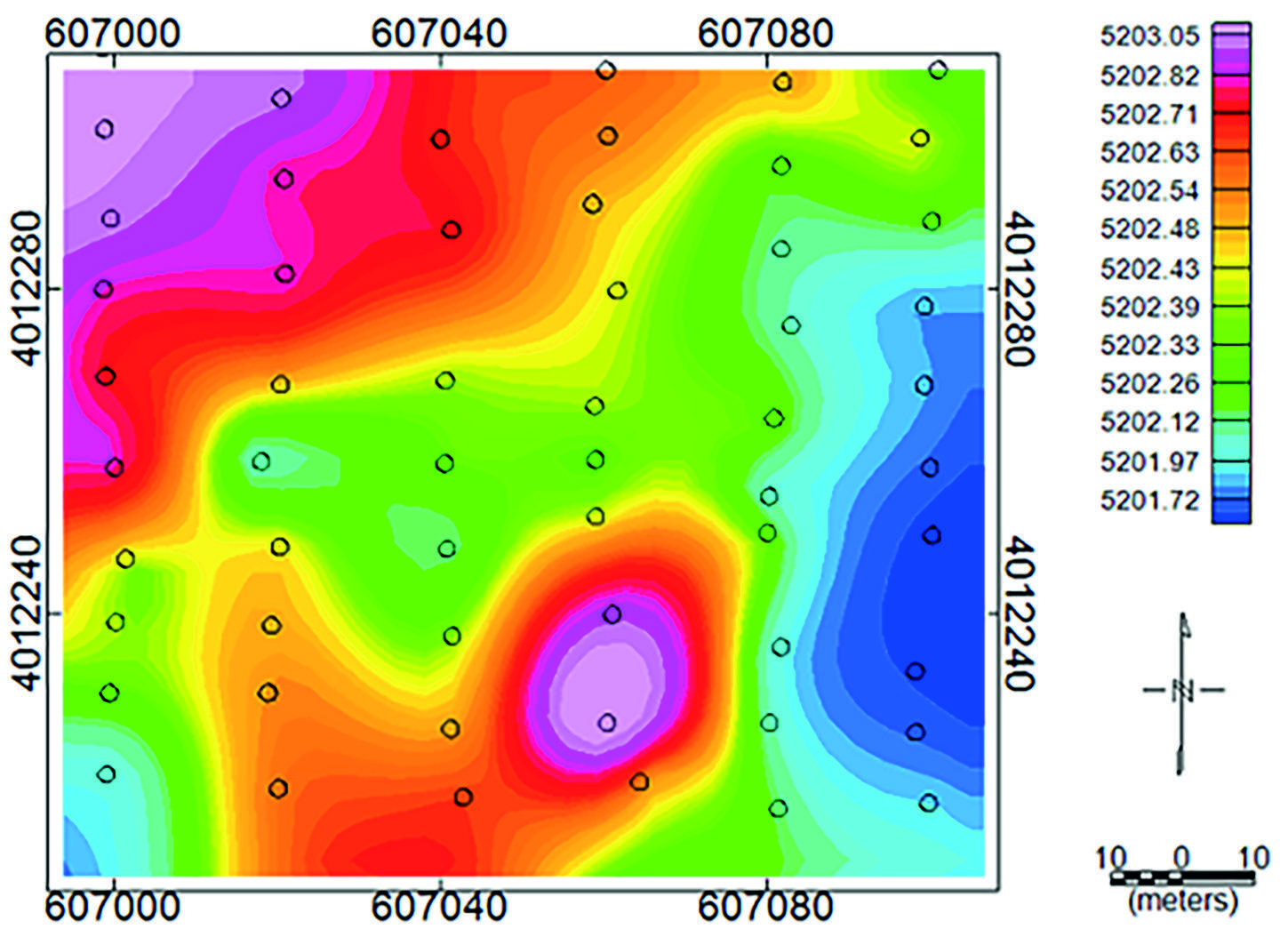
Figure 13. Bouguer gravity field map of the area under investigation as the gravity reading stations have been shown on it by the black circles.
Therefore, it is necessary to remove the regional field from the Bouguer gravity field using the 2-degree surface trend method so that the residual gravity anomaly will be obtained. Almost, all the qualitative and quantitative analyses are performed on the residual gravity field.
Figure 14 shows the produced residual gravity field using the second-degree surface trend. Due to the high density difference between the Chromite host rock and the surrounding rocks, we expect chromite-bearing zones to be highlighted on the residual gravity anomaly map with a positive gravity value. As seen in the residual gravity anomaly map in Figure 14, a region with the maximum positive gravity field value has been detected in the southern part, which most likely has a source body that forms the chromite host rock.
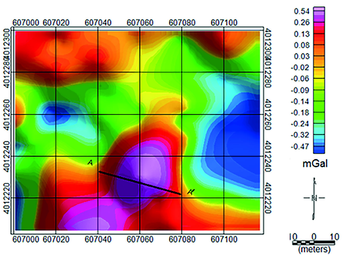
Figure 14. The residual gravity map of the area under investigation. The location and direction of the profile AA' has been shown on the positive gravity anomaly.
For 2-D modeling of the subsurface causative mass, we analyze the residual gravity field variations along the profile AA' which runs across the Chromite mineral mass in an approximately W-E direction as is shown in figure 14. Data sampling has done in 11 points with an interval of 4 m over the profile AA' with a length of 40 m.
4.3 Analysis of Gravity Horizontal Gradient
To analyze the real gravity horizontal gradient along the profile AA (green curve in Figure 16(a)) using the reweighting focusing inversion, the number of iterations and the value of 2-norm errors between the observed gravity horizontal gradient and inverted ones were set to 25 repetitions and 0.0001 mGal/m, respectively.
Figure 15 shows the changes of 2-norm errors with the increase in the number of iterations. The 2-norm values reached 0.00015 in the 12th iteration and obtained 0.000074 in the 13th iteration, which is lower than the initial assumed error value.
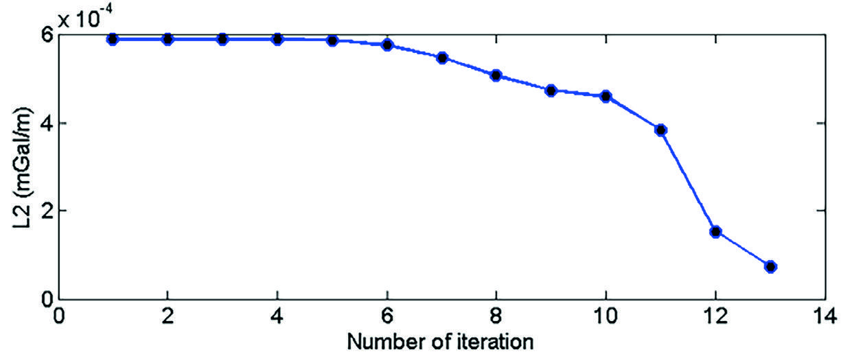
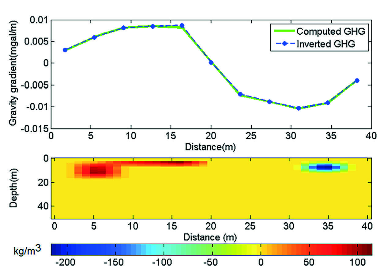
Therefore, the optimized inverted response belongs to the computed density distribution in the 13th iteration. The variations of the gravity horizontal gradient corresponding to the recovered density contrast distributions of the inversion is shown in figure 16(b) as is depicted with the blue dashed curve in Figure 16(a). As seen in Figure 16(a), a mass with negative values has been located at a depth about 5 meters, 33 meters from the first data sampling point, and another one with positive values has been settled at a depth between 5 to 10 meters, approximately 7 meters far from the starting point. Based on the obtained results, the maximum horizontal expansion of the anomaly source is around 26 meters.
5. Detection of the Gravity Anomaly Border Using the Conventional Methods
In this chapter, three common edge detector filters namely analytic signal, tilt angle, and total horizontal derivative were used to detect the anomaly source edges as we can compare these results with the estimated border from the reweighting focusing inversion method. Because these filters are applied on the gridding of the gravity field, we can determine the horizontal expansion of the subsurface source through analysis of the obtained maps from these edge detection filters.
5.1 Analytic Signal
Nabighian developed an automated method for the interpretation of 2-D magnetic anomalies based on the analytic signal in some articles from 1972 to 1974. The maximum value of the analytic signal take place on the anomaly causative mass. Using this property of the analytic signal, the location of the source and its edges can be detected. The analytic signal function for the gravity data (T) is defined as:
Figure 17 shows the analytic signal map for the study area. As was mentioned, the maximum values of the analytical signal are located on the anomaly source. We have considered values greater than 0.05 mGal/m as the maximum values of the analytical signal filter. As depicted in Figure 17, a contour line of 0.05 mGal/m has been drawn around the anomaly related to the chromite mass, which is assumed to be the border of the subsurface source. The dashed line shown in Figure 17 almost corresponds to the direction of profile AA' The length of this dashed line is approximately 25 meters. Therefore, the distance between the edges of the anomaly source along this dashed line is about 25 meters, which closely matches with the distance of the edges which estimated by the inversion method (26 meters).
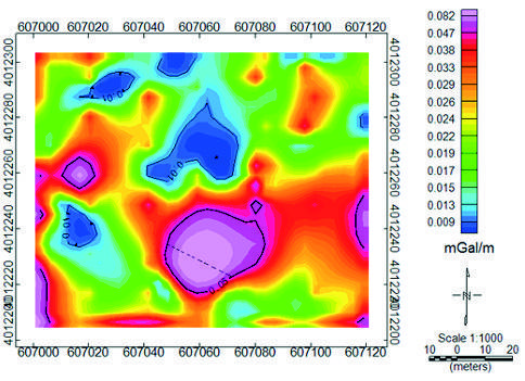
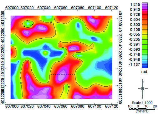
5.2 Tilt Angle
A prevalent local phase filter is the tilt angle (deviation angle) (Miller and Singh, 1994) which can be easily computed for both frequency and the space domains, and is defined as follows:
Where f is gravity or magnetic field. The tilt angle gradient has interesting properties. As a dimensionless ratio, it responds very well to deep and shallow sources and has a wide range of variations for sources at the same level. For a source with positive density, the tilt angle is above the positive anomaly. Near the edges, where the vertical derivative is zero and the horizontal derivative is the largest, the value of the tilt angle is zero, and outside the subsurface anomaly zone, it is negative.
Figure 18 shows the tilt angle of the study area in Sabzevar. The contour line with the zero radian indicates the border of the subsurface sources, as has been drawn on the tilt angle map in figure 18. As observed in Figure 18, the tilt angle filter could not separate a confined part as the border around the gravity anomaly related to the chromite mass. However, since the zero values of tilt angle detect the anomaly source edge, we have connected these values in the east-west direction on the anomaly by a dashed line (Figure 18). This line is 30 meters long which indicates that the horizontal expansion of the subsurface anomaly source in the east-west direction is 30 meters. Although the direction of the dashed line in Figure 18 is not in the same direction as profile AA', the value of the area for the subsurface mass obtained by the tilt angle is acceptably close to the value obtained by the reweighting focusing inversion method.
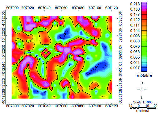
5.3 Total Horizontal Derivative:
The maximum value of horizontal derivatives, which is also known as the total horizontal derivative which leads to better detection of anomaly edges in any direction, is defined as follows (Cooper, 2006):
Figure 19 shows the map obtained from the total horizontal derivative executed on the gravity data related to the study area in Sabzevar. Similar to the tilt angle, this filter also has failed to create a closed curve of its maximum values around the positive anomaly of the chromite mass as the source edge, and it could not detect a specific border. The curve with the same contour of 0.1 mGal/m is shown on the total horizontal derivative map. The maximum values of this filter are located in the middle of this level curve. Similar to Figure 18, a dashed line in the east-west direction connects the maximum values between the 0.1 mGal/m contour lines that correspond to the mass border. This line, which indicates the distance between the eastern and western borders of the mass, is around 34 meters long. Therefore, this filter has estimated the horizontal outspread of causative mass 8 meters higher than the value obtained from the reweighting focusing inversion method.
6. Estimation of Chromite Mass Depth
In this chapter, two common depth estimation methods, namely the Euler Deconvolution and power spectrum (energy density spectrum) methods are used to estimate the depth of the chromite mass. Figure 20 shows the estimated depth by the Euler deconvolution method for a 5x5 window length on the residual gravity field. As seen in this figure, the depth of the top surface of the chromite mass is between 5 to 10 meters.
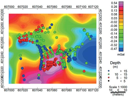
Figure 20. Resulted depth by the Euler Deconvolution method drawn on the residual gravity field map.
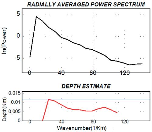
The power spectrum method estimates the average depth of the top surface of the anomaly source mass about 11.5 meters (the intersection of the horizontal blue line with the depth axis in Figure 21). It should be noted that the power spectrum method uses all the existing wavelengths for estimation of the depth of the top surface of the source masses in the study area, so the overestimation of the depth of the top surface is expected.
7. Non-linear Inverse Modelling
To obtain the shape of the subsurface chromite mass, we used Model Vision software for a two-dimensional non-linear inversion of the gravity field along a profile with a 100 m long. which was almost in the same direction with the profile AA'. Data sampling was done at 11 points at a distance of 10 meters in the direction of the gravity profile. The black curve in Figure 22 shows the gravity field changes along this profile. The structure obtained from the nonlinear inversion for the underground mass is shown in Figure 22. The blue curve in Figure 22 shows the inverted gravity field corresponding to the subsurface mass. Also, the obtained 2-norm error between observed and computed gravity values is 0.41 mGal/m
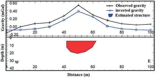
Based on Figure 22, the depth of the top surface of the mass is around 5 meters and the highest value of the horizontal expansion is 21 meters. The eastern border of the mass is shown as a point at a depth of 5 meters, and the western border is a vertical line, almost 7 meters long (5 to 12 meters deep).
8. Conclusion
Analysis of the synthetic models indicates that the use of gravity horizontal gradient data in the reweighting focusing inversion algorithm produces distributions of positive and negative density which correspond to the farthest vertical borders of subsurface mass, and can relatively estimate the deep expansion of the mass. The efficiency of the suggested method in the present study in revealing the underground anomaly source mass border was investigated with two synthetic models. The results indicate that density distributions obtained from the reweighting focusing inversion algorithm are well focused on the top part of the subsurface structure edges with the highest distance. Thus, by the use of this method, the underground depth and location of the farthest edges of an underground structure can be detected.
The inversion method was used for the analysis of the gravity horizontal gradient of a chromite mass. The density distributions estimated a depth of 5 meters for the eastern edge and 5 to 10 meters for the western edge of the subsurface mass, which are approximately similar to the results obtained by the non-linear inverted modeling (Figure 22). Three common edge detection filters were used for validation, which estimated the horizontal expansion of subsurface mass to compare with the value obtained from the inversion (26 meters). The conventional depth estimation methods have estimated the depth of the top surface of the chromite mass in the range between 5 to 10 meters. Therefore, the location of the subsurface density distributions is almost correspondent to the top surface of the mass. Also according to the results, it can be concluded that the highest horizontal expansion belongs to the top surface of the mass. The non-linear inverse modeling also estimated the expansion of the top surface of the subsurface mass about 21 meters which show a good conformity with the obtained result from the proposed method. It should be noted that the analyses made for the depth and expansion evaluation of the underground mass are related to the direction of the data sampling profile.
The use of the method developed in the present study, alongside other qualitative and quantitative maps, can effectively help the analyzer with the analysis of the gravity field and detection of the parameters of the underground structure.

