1. Introduction

Seismic observations are serving as a major source of the current knowledge on tectonic processes in the Earth. The main object of interest is the earthquake: its location and source mechanism are interpreted in terms of global or local geological models. The earthquake location is an answer on the question “where” and acting as a source of the related fault geography. The earthquake mechanism is used as an answer on the question “how” this fault acts. The so-called double-couple (DC) mechanism is the most common interpretation of the analyzed seismic amplitudes. It has a clear physical interpretation of being equivalent to a shear faulting along a plane segment. Moreover the analysis is sometimes reduced to “beach-ball” diagram analysis, when instead of wave amplitudes analysis only the sign of the arrival is analyzed. Many field data results show more general moment tensors with significant non-double-couple (non-DC) components. Such non-DC mechanisms include a cavity collapse in mines (^{Sileny and Milev, 2008}), and tensile faulting induced by fluid injection in geothermal or volcanic areas (^{Julian et al., 1998}). In some applications one can expect that the non-DC mechanisms should prevail. For example, hydraulic fracture treatment implies a fracture opening which should produce tensile (dipole-type) sources (^{Sileny et al., 2009}), along with double-couple sources (^{Nolen-Hoeksema and Ruff, 2001}).

Recent years have brought a better understanding of geomechanic processes in the geologic materials including rock deformation and failure (e.g. see ^{Zoback, 2010}). Numerical modeling is used for the analysis of deformation and stress field around magma chambers (^{Currenti and Williams, 2014}), for prediction of fracture zones (^{Maerten et al., 2006}) etc. Starting from the classic linear-elastic fracture mechanic models, many complicated geomechanic modeling methods have been developed for simulating the development and propagation of the fracture accounting for the whole complexity of real geologic formations, plastic failures and fluid/rock interactions (^{Wang et al., 2016}; ^{Flekkøy et al., 2002}). It is generally accepted that linear fracture geometries are formed in the ductile formations while complex and interconnected discrete fracture networks are formed in more brittle formations. Another crucial aspect is modeling of the main fracture interaction with other natural fracture systems (^{Zangeneh et al., 2014}). Simulation results demonstrate that final fracture-pattern complexity is strongly controlled by anisotropy of in-situ stresses, rock toughness, orientation of the natural fractures and their cement strength (^{Dahi-Taleghani and Olson, 2011}). The complexity of seismic source mechanism is enhanced when main fracture may hit pre-existing fractures resulting in a shear-type displacement as well (^{Maxwell, 2014}). Note that numerical simulations show that the growing fracture may exert enough tensile and shear stresses to re-open even cemented natural fractures (^{Dahi-Taleghani and Olson, 2011}). However, the link between tectonic processes or production practices is complicated and not yet well-understood. Connection between observed earthquakes and models of rock failure is not simple in most practical cases. Recent theoretical developments in both fields (seismic data inversion and geomechanic modeling) require additional effort in establishing a connection between them.

The fluid’s role in earthquakes sometimes seems to be underestimated. Laboratory experiments show that the injection fluid viscosity should influence the fracture propagation detectable by acoustic observations, e.g. viscous fluid injection tends to generate thick and planar cracks producing shear-type mechanisms, less viscous fluid results in thin and wavelike cracks producing tensile-type mechanisms (^{Ishida et al., 2004}). A growing amount of seismic data observed for hydraulic fracturing monitoring allows establishing empirical relations between the parameters of seismicity and hydraulic fracture propagation (^{Warpinski, 2013}). Seismic moment-tensor inversion results are also used for constructing the dominant fracture sets that can provide constraints on the rock properties controlling the fracture growth in the reservoir (^{Baig and Urbancic, 2012}). Integrated fracture system simulation, monitoring, and model updating for reservoir development are discussed in detail in (^{Pettitt et al., 2011}; ^{Maxwell et al., 2015}).

However, note that seismic moment-tensor inversion is related to radiation pattern analysis which is also affected by media parameters which are seldom taken into account, and the media considered as homogeneous and isotropic. For example, the radiation pattern may be considerably influenced by seismic anisotropy in the area of the source (^{Psencık and Teles, 1996}), the so-called directivity effect caused by unilaterally rupturing fault (^{Lay and Wallace, 1995}), also see the review by ^{Julian et al. (1998)}). ^{Shi and Ben-Zion (2009)} consider radiation patterns for the cases of the similar and dissimilar solids on the sides of the fault and, with numerical modeling, analyze radiation patterns and their possible interpretation in terms of source mechanism. Many potential distorting factors should be taken into account during geologic interpretation of the seismic inversion results. The problem of connecting effective seismic moment tensors to actual seismic emission from the rock failure was first addressed by ^{Loginov et al. (2016)}. Here we consider it in more details.

In this paper we perform a numerical geomechanic modeling of different scenarios of the incremental fracture growth based on the elastic-plastic model of the rock deformation and failure in the form of the fracture growth. This modeling includes the generation and propagation of elastic waves. These waves are analyzed in order to approximate them by an effective point seismic source that is a natural interpretation of the observed seismic events. These results will be used for connecting the geomechanic models of fracture propagation to the moment tensors that can be retrieved from a seismic data.

2. Theory

3. Numerical Tests

In this section we will show the results of a series of numerical simulations of different scenarios of the incremental fracture growth. Associated seismic emission is then compared to the tensor-moment solutions as suggested in (^{Loginov et al., 2016}).

The model of the incremental fracture growth as schematically shown in Figure 1,A. The main fracture extends from the bottom up with its tip being in the center of the computational domain. In all simulations we consider homogeneous material with the following properties: density is 2.5 kg/cm³, P-wave velocity is 6 km/s, and S-wave velocity is 3.34 km/s, Y=15 MPa, α=0.5,β=0.2. We assume fluid inside the fracture in case of its opening, i.e. there is no material with altered properties but pressure is applied to the fracture surface as a boundary condition.

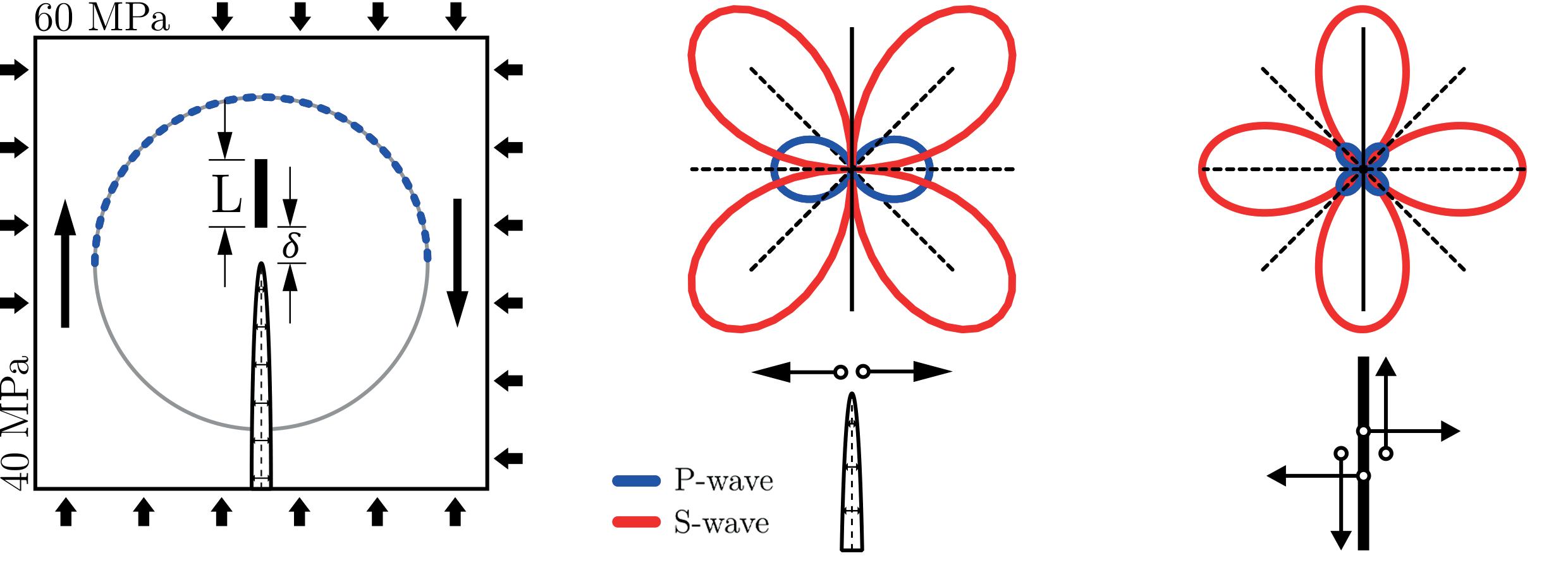
Figure 1. Fracture elementary growth scenarios. A) - geomechanic modeling domain, main fracture and possible pre-existing crack in front of it, arrows show the confining stresses, grey circular - receiver profile, blue dotted half-circle- receiver line used for the moment-tensor inversion; B) - radiation pattern for tensile fracture opening; C) - radiation pattern for shear-type fracture growth. P-wave - blue, S-wave - red. 

Confining stress (emulating regional stress field) was applied at the boundaries (as schematically shown in Figure 1,A). In all experiments 40 MPa normal stress was applied to the side boundaries, while 60 MPa normal stress was applied to the top and bottom boundaries (so that the main fracture is aligned with the maximum normal stress direction). In some of the experiments we also applied the shear stress to the side boundaries (10 and 30 MPa). The fracture growth may take place in a continuous homogeneous medium or it may hit a preexisting co-linear crack of length L. Generated elastic wavefields are recorded on a circular profile centered at the main fracture tip. The radius (150 or 200 m) is chosen so that the profile is in the source far field, i.e. P- and S-waves are formed and well separated.

All scenarios of the main fracture advancement include its incremental growth to the length δ (see Figure 1,A). This growth may have a tensile-type mechanism caused by a pressure inside the main fracture (mimics hydro-fracturing). Corresponding radiation patterns of P- and S-waves are shown in Figure 1,B (dipole-type source). Alternative scenario of the fracture growth is a shear-type mechanism caused by the boundary shear stress (mimics fault activation). Corresponding radiation patterns of P- and S-waves are shown in Figure 1,C (double-couple source).

In Figure 2, left we show the elastic wavefield generated by the main fracture incremental growth (δ=3 m) due to tensile opening in continuous medium (no pre-existing crack). One can see traces from 100 receivers placed on the circular profile: radial displacement velocity component (with respect to the main fracture tip) is shown in the top panel, transversal component – in the bottom panel. The horizontal axis shows the receiver angle on the circle (measured from the vertical axis so that the profile crosses the main fracture at angle π). One can see the P- and S-waves on the radial and the transversal components correspondingly. Central traces clearly contain the Rayleigh wave propagating along the walls of the main fracture. Particle motion trajectories (hodograms) are shown in Figure 2, right. Trajectories of the particle motion for P-wave are shown in blue (they correspond to the time interval of P-wave shown by blue horizontal lines in Figure 2, left); trajectories for S-waves are shown in red (correspond to the time interval of S-wave shown by red horizontal lines in Figure 2, left). One can see that the polarization of both waves is close to linear which is expected for a point source in elastic medium.

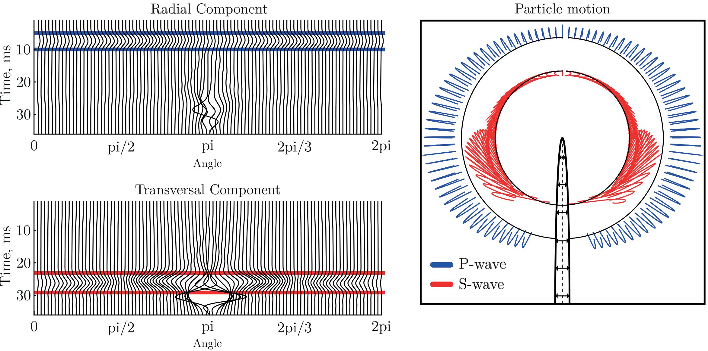
Figure 2. Elastic wavefield generated by the fracture tensile opening (no pre-existing crack, normal boundary stresses). Left: wavefield recorded on the circular line (cf. Fig. 1), radial component of particle velocity - top panel, transversal component bottom, windows of polarization analysis are shown for P-wave (blue lines) and S-waves (red lines). Right: particle motion trajectories for the time intervals of P-wave (blue) and S-wave (red). 

As mentioned earlier while modeling the main fracture incremental growth at distance δ we disconnect nodes of the computational grid but we release the new fracture borders continuously with some prescribed speed. In Figure 3 we show the results of using different border release speed.

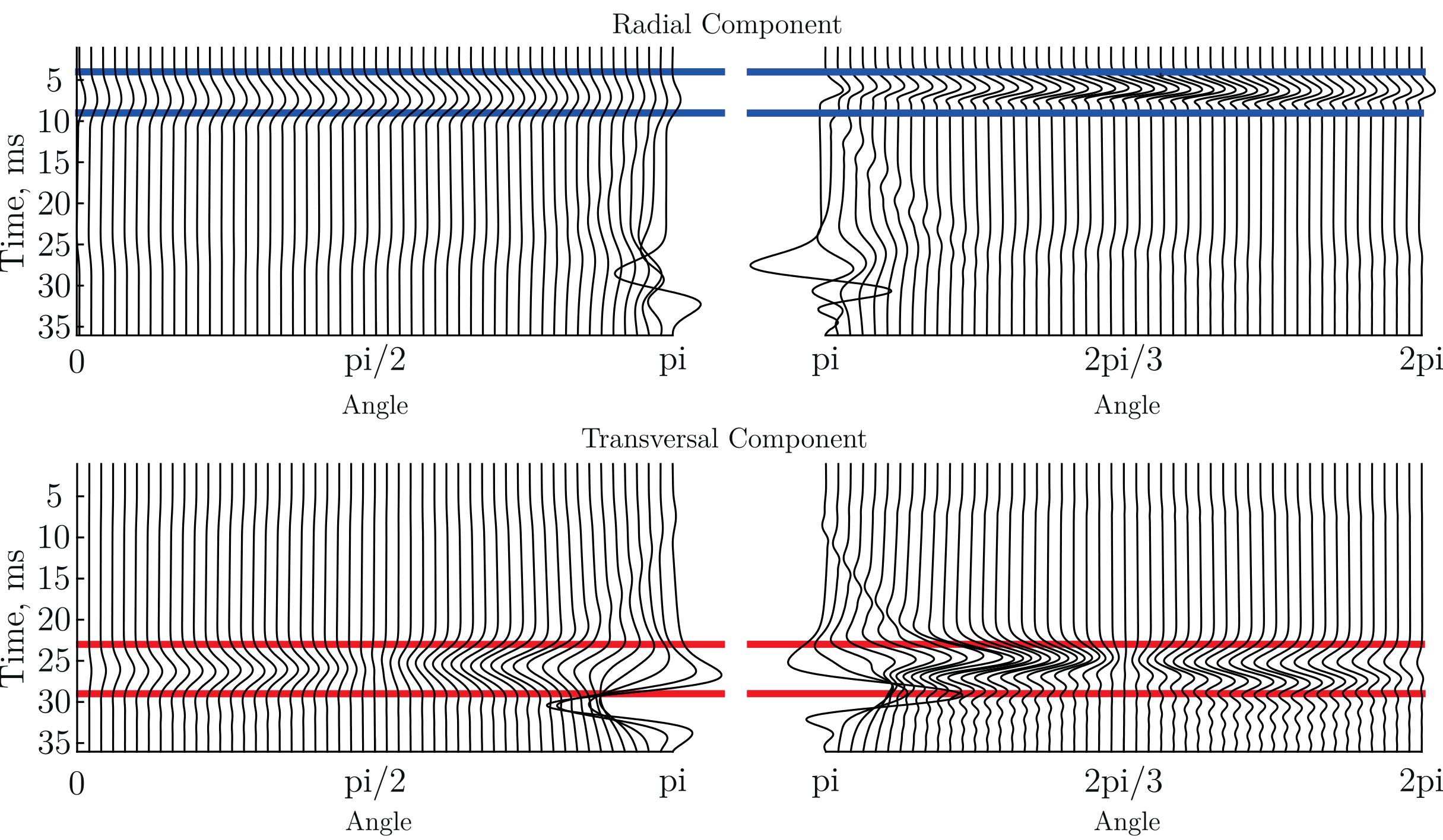
Figure 3. Elastic wavefield generated by the fracture tensile opening with a different speed (no pre-existing crack, normal boundary stresses) and recorded on the circle from Figure 1: top radial component; bottom - transversal component. Left: slow opening speed; right: fast opening speed. 

Now we consider the same fracture advancement δ=3 m but different border release speed, as shown in Figure 3. Right panels correspond to the release speed 4 times faster than for traces in the left panels. One can see that faster fracture opening generates waves with higher amplitudes and shorter signal periods. Here we get the P-wave wavelength about 30 m for the data in Figure 3, left and about 15 m for Figure 3, right. Then we pick P-wave amplitudes as the maximum absolute values of the radial component within the P-wave time interval (blue lines in Figure 3); S-wave amplitudes are picked on the transversal component within the S-wave time interval (red lines in Figure 3). Corresponding radiation patterns are shown in Figure 4: blue - for P-waves, red - for S-waves. They show absolute values of waves radiated in all directions assuming that they were generated by a point source located at the fracture tip. One can see that faster border release produces stronger waves but overall shape of the radiation pattern is similar. Thus for further experiments we choose the border release speed which produces cleaner traces (without oscillating numeric dispersion).

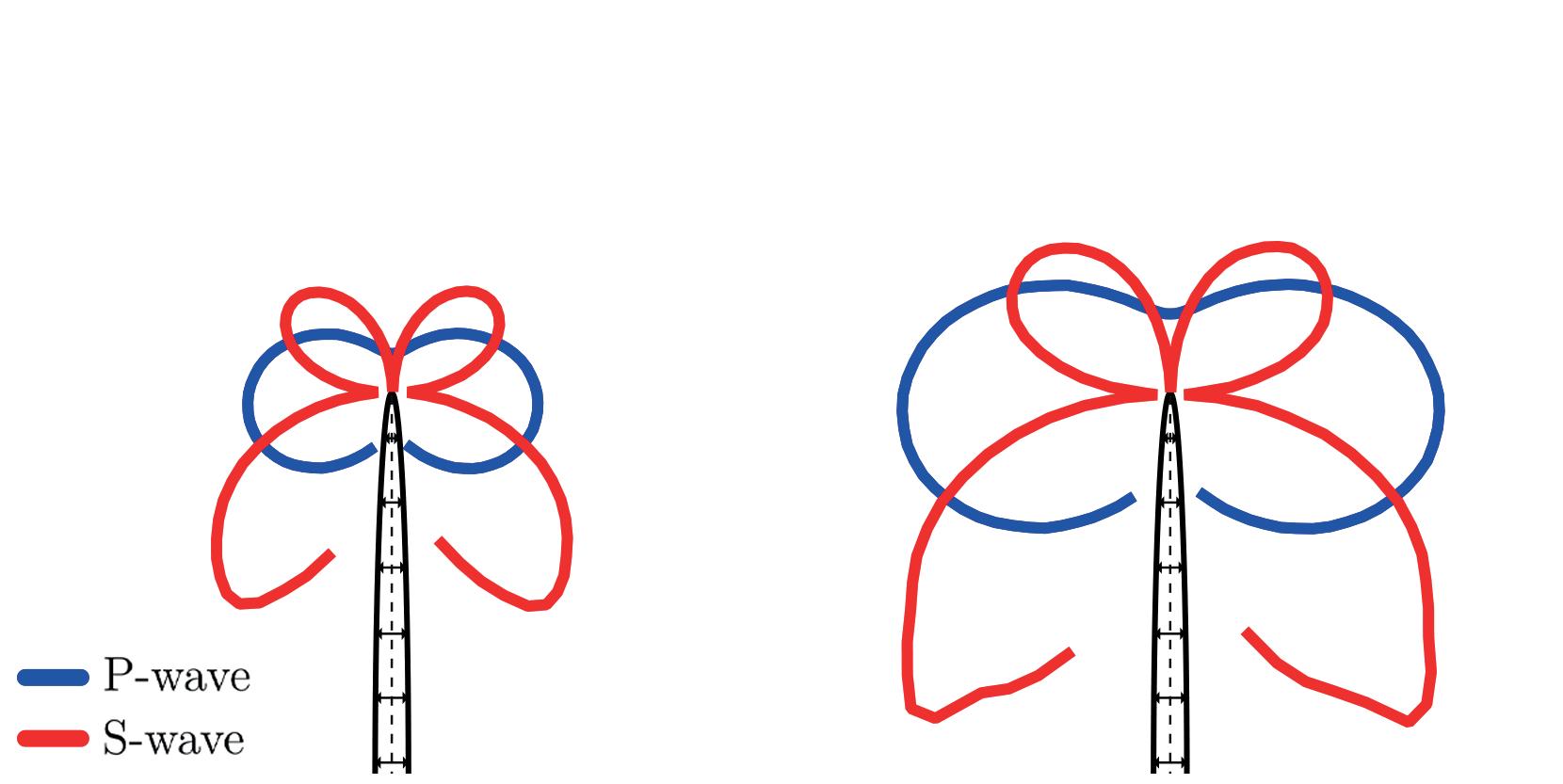
Figure 4. Radiation patterns for the fracture tensile opening with a different speed (no pre-existing crack, normal boundary stresses); blue - P-wave; red - S-wave. Left: slow opening speed; right: fast opening speed. 

Now let us consider the case when advancing fracture breaks the ‘bridge’ towards preexisting small crack as schematically shown in Figure 1. In Figure 5 we show the radiation patterns for the fracture tensile opening in the case normal boundary stresses; blue lines – P-wave; red lines – S-wave. Three model results are shown: no pre-existing crack (A); pre-existing crack of length 10 m (B); crack of length 20 m (C).

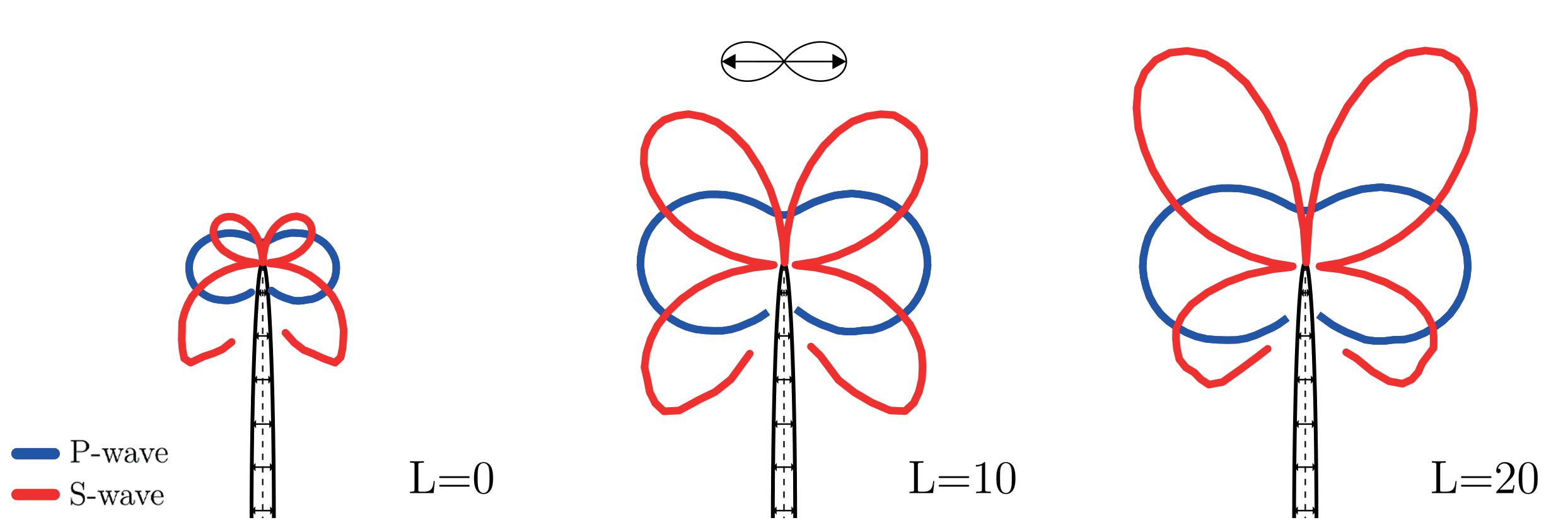
Figure 5. Radiation patterns for the fracture tensile opening in case of pre-existing cracks of different length (normal boundary stresses); blue - P-wave; red - S-wave. A) - no pre-existing crack; B) - crack of L=10 m; C) - crack of L=20 m. 

Let us make a few observations from these results. Note that in most cases the S-wave radiation pattern differs from the ideal one known for the dipole point source (cf. Figure 1). Fracture incremental growth in continuous medium results in more S-wave energy radiated back toward the fracture origin (Figure 5,A). This may be an effect of the fracture walls during the wave formation in the near-zone of the source. Stronger waves are generated when the main fracture hits a pre-existing crack. Moreover, the radiation patters changes. Now more energy of the S-wave is emitted forward, i.e. in the direction of the fracture growth. One can see that for some crack length the radiation pattern starts resembling the ideal dipole source (Figure 5,B); then it becomes non-symmetric again (Figure 5,C), note the similar analytical observation in ^{Aki and Richards (2002, Chapter 10, Figure 10.20)}. Also note that the horizontal orientation of the dipole derived from the radiation pattern coincides with our expectations of the tensile opening of the fracture.

Now we consider the case the shear boundary stress added to the normal boundary stress and the tensile mechanism of the fracture growth. Corresponding radiation patterns are shown in Figure 6 for the shear boundary stresses of 10 MPa (bottom row) and 30 MPa (top row). As usual, blue lines correspond to P-waves, red lines – to S-waves. Note that at the boundaries we now add shear stresses (at the sides) to the normal stresses (cf. Figure 1). Thin lines show orientations of the principal stresses of the resultant stress field. Columns in Figure 6 correspond to different length of the pre-existing crack: no crack (A, D), L=10 m (B, E), L=20 m (C, F).

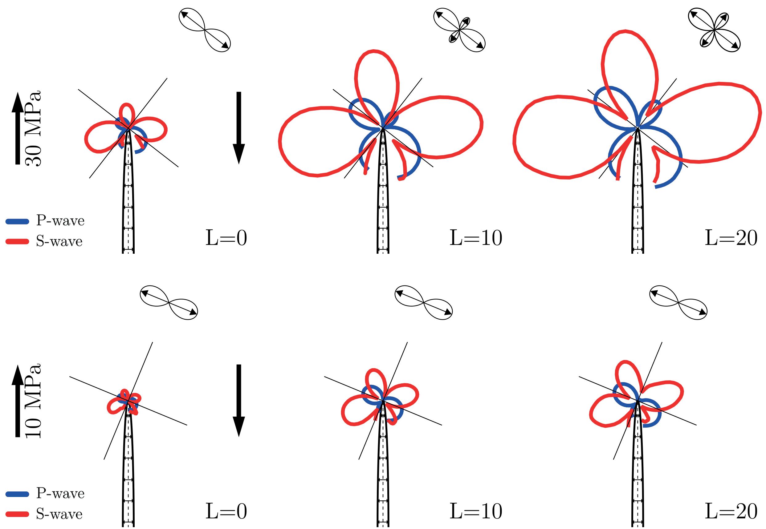
Figure 6. Radiation patterns for the fracture tensile opening in case of additional shear boundary stresses of 10 MPa (bottom row) and 30 MPa (top row). Columns correspond to different length of the pre-existing crack: no crack (A, D), L=10 m (B, E), L=20 m (C, F). Thin lines principal stress orientations due to boundary stresses. P-wave - blue, S-wave - red. 

In Figure 6 one can see that the intensity of generated waves increases when value of the shear stress increases (from the bottom up) or length of the pre-existing crack increases (from left to right). In the panels we also show how the P-wave radiation pattern can be interpreted in terms of the dipole sources (the S-wave radiation pattern is more complicated and deviates more from the ideal patterns). Note that small shear stress rotates the stress orientations. And the radiation patterns derived from seismic waves correspond to the rotated dipole aligned with these stresses instead of the fracture growth direction (Figure 6, bottom row). For larger boundary shear stress the stress orientations are rotated even more. The P-wave radiation patterns are still aligned with these directions but they are do not look like corresponding to a pure dipole type (Figure 6, top row). They start looking like a rotated double dipole source which will further transform into a double-couple source for even stronger boundary shear stresses.

Then we consider pure-shear rock failure at the fracture due to 30 MPa shear boundary stress (no pressure in the fracture, the same normal boundary stresses). Radiation patterns corresponding to different length of the pre-existing crack are shown in Figure 7: no crack (A), L=10 m (B), L=20 m (C). As usual, blue lines correspond to P-waves, red lines – to S-waves. Note that the S-wave radiation pattern is asymmetric and differs from the ideal double-couple source (Figure 1,C). With the increasing length of the pre-existing crack we see the increasing intensity of generated waves and the S-wave radiation pattern becomes less asymmetric.

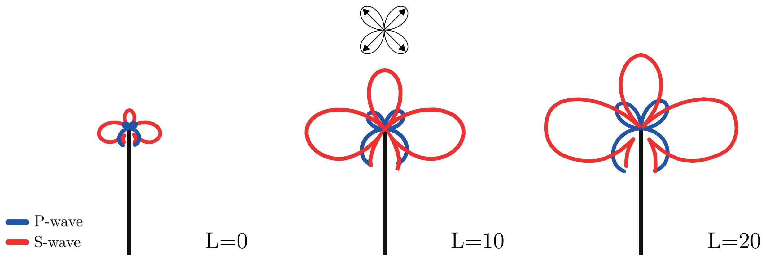
Figure 7. Radiation patterns for the fracture shear-type development (no pressure in frac-ture, 30 MPa shear boundary stress) for different lengths of pre-existing crack: no crack (A), L=10 m (B), L=20 m (C). P-wave - blue, S-wave - red. 

Finally we applied the seismic moment-tensor inversion (SMTI) to the picked P- and S-wave amplitudes. In order to avoid influence of the Rayleigh wave propagating along the fracture we consider restricted aperture of the acquisition array shown by dashed blue line in Figure 1 (upper half-circle). We present the inversion results in Figure 8. Solid lines show the radiation patterns from our geomechanic modeling, dashed lines – the moment-tensor inversion. Panels correspond to different scenarios of the fracture growth.

One can see that overall the radiation pattern observed from geomechanic modeling can be reasonably well approximated by a moment-tensor point source. Inversion results fit the P-wave radiation pattern almost perfectly. Some misfit can be seen for the S-wave radiation pattern in the case of considerable shear boundary stress (30 MPa). In this case the modeling result show stronger S-wave radiation in the direction orthogonal to the main fracture compared to the forward direction (note that the ideal double-couple mechanism produces symmetric sectors of the S-wave radiation pattern, cf. Figure 1,C).

First we consider the tensile fracture opening in the case of normal boundary stresses, and the pre-existing crack of length L=10 m (Figure 8,A). The moment-tensor inversion gives us the radiation pattern which is very close to the theoretical dipole-type source (cf. Figure 1,B) which is a natural mechanism for this case. The dipole orientation perfectly identifies the fracture growth direction (should be orthogonal to the dipole orientation). Then we consider the tensile fracture opening in the case of small shear boundary stress (10 MPa), and the pre-existing crack of length L=20 m (Figure 8,B). Note that the source mechanism still looks very much like a dipole but it is oriented at an angle of 22° from the horizontal. Thus the dipole source orientation provides false information if it is interpreted as showing the fracture growth direction (corresponds to the principal stress directions). Next we consider the tensile fracture opening in the case of stronger shear boundary stress (30 MPa), and pre-existing crack of L=20 m (C) (Figure 8,C). Note that the P-wave radiation pattern now corresponds to two orthogonal dipoles of different intensity oriented at an angle of 37° from the coordinate axes. The S-wave radiation pattern is not fitted perfectly and it exhibits asymmetry of radiation discussed earlier for the shear-type mechanism. Note that now the tensile nature of the fracture opening is somewhat masked in the source mechanism and its orientation is not showing the fracture growth direction. Finally, we consider the shear-type fracture development in the case of shear boundary stress (30 MPa), and pre-existing crack of L=20 m (C) (Figure 8,D). Note that the P-wave radiation pattern is well fitted by the double-couple mechanism, while the S-wave radiation pattern is not fitted perfectly and it exhibits asymmetry of radiation discussed earlier for the shear-type mechanism. Also note that if this mechanism is interpreted as a double-couple (cf. Figure 1,C) then its orientation is in good correspondence with the fracture growth direction.

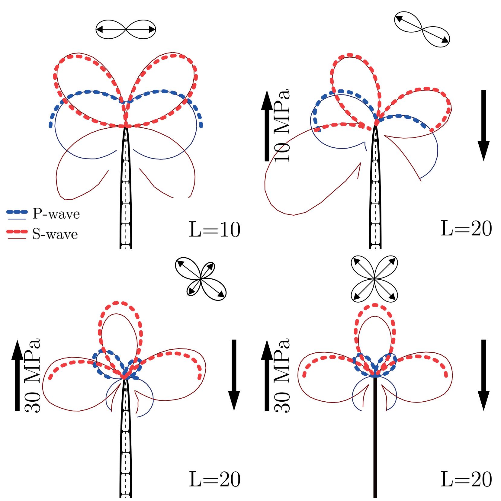
Figure 8. Seismic moment-tensor inversion results for different models; solid line - radiation pattern from geomechanic modeling, dashed line - the moment-tensor inversion result. Different scenarios of the fracture growth: tensile opening, only normal boundary stresses, pre-existing crack of L=10 m (A); tensile opening, 10 MPa shear boundary stress, pre- existing crack of L=20 m (B); tensile opening, 30 MPa shear boundary stress, pre-existing crack of L=20 m (C); shear-type growth (no pressure in fracture), 30 MPa shear boundary stress, pre-existing crack of L=20 m (D). P-wave - blue, S-wave - red. 

4. Conclusions

This study explores the limits of seismic monitoring’s theoretical ability to resolve rock failure mechanisms associated with fracture growth or activation. Our approach includes numerical geomechanic modeling of incremental rock failure (fracture growth) accounting for elastic wavefield generation and propagation. We record this wavefield and perform its seismic processing (seismic moment-tensor inversion). In this way we get effective point-source mechanisms which can be associated with earthquakes observed during fracture propagation.

Then we try to establish connections between the moment tensor solutions and different geomechanic scenarios of the fracture development. For this we carry out numerical geomechanic simulations corresponding to different scenarios of elementary fracture growth (small advancement step): different fracture growth mechanisms (tensile and shear), different types of boundary stress (only normal stress, normal and shear stresses), interaction with pre-existing cracks. We then check if these scenarios can be identified from elastic waves recorded in a far field of the source.

In general, amplitudes of generated elastic waves can be reasonably well approximated by moment-tensor point sources. Especially for the tensile-type fracture growth (fracture opening due to excessive pressure in it) we usually get radiation patterns corresponding to dipole-type source mechanisms which is in good agreement with the theory.

Let us sum up a few more observations. Note that when the fracture hits a pre-existing crack then stronger waves are generated compared to the fracture growth in continuous medium. Thus our modeling confirms the concept that the fracture growth itself may take place without producing much seismicity while noticeable earthquakes may be generated when the main fracture hits pre-existing cracks and faults (cf. ^{Maxwell, 2014}). However, we have got some new observation about the shape of the radiation patterns in this case. We noted that for the tensile fracture growth in homogeneous medium there is more S-wave energy radiated backward (towards the fracture beginning). For the fracture hitting the pre-existing crack we see some compensation of this effect. So that the radiation of the S-wave forward increases with the increasing length of the pre-existing crack. Thus at certain crack size the S-wave radiation pattern appears to be close to the theoretical one for the dipole source (tensile fracture opening).

Note that the described asymmetries in the radiation patterns may cause distortions in the magnitude estimations depending on the acquisition design. Also note that there are other sources of such asymmetries discussed in the introduction. We hope that it is possible to distinguish between these different sources. For example, the influence of seismic anisotropy is reported to have stronger affect on the P-wave radiation pattern (cf. ^{Psencık and Teles, 1996}) while our experiments show that the S-wave radiation pattern is affected more. The directivity effect from rupturing fault (^{Lay and Wallace, 1995}) results not only in the distortion of the radiation pattern, but the signal period should be also different in different directions. We do not see such signal variability in our data.

Finally, our examples show that seismic moment-tensors may give a completely wrong estimation of the direction of the fracture growth (advancement). Inverted mechanisms of the dipole type are usually associated with the fracture tensile opening (being orthogonal to the fracture advancement direction). But the dipole orientation may differ considerably from the fracture growth direction in presence of shear boundary (regional) stresses. This result should be kept in mind when interpreting seismic data.

We hope that further studies will help establishing better connections between geomechanic models of rock failure and the inversion of seismic data. Then the seismic observation may be successfully used for calibrating geomechanic models with applications in monitoring hydraulic fracturing, reservoir development and regional tectonic processes.