


 nueva página del texto (beta)
 Inglés (pdf)
 Artículo en XML
 Referencias del artículo
 Enviar artículo por email
 Citado por SciELO
  Similares en
SciELO
Similares en
SciELO 
 Permalink
1. Introduction
The air temperature is an indicator of the structure, functionality, and geographic location of environmental systems and plays an essential role in biological and ecological functions. Similarly, body temperature is a crude indicator of basal metabolism (Protsiv et al., 2020). The environmental air temperature depends on latitude (Fuelner et al., 2013) and altitude (Hemond and Fechner, 2015; Isaak et al., 2018; Chen et al., 2018) and is influenced by many factors (Sun, 2016), such as time on day, weather, surface type, geographical location, and elevation. Therefore, the spatial and temporal study of the air temperature and their relationship to the anthropic environment modifications are of great interest as urban areas and land-use change. Furthermore, temperature increase can dramatically affect the cells of living organisms and the populations, with ecological consequences (Waldock et al., 2018), by altering the relationships between biodiversity and the functioning of ecosystems (García et al., 2018), increasing the respiration rate and decreasing the plants' photosynthesis (Duffy et al., 2021).
The effect of environmental modifications on air temperature has been analyzed by comparing rural and urban areas or their surroundings; in places where buildings abound, the temperature is higher than in other areas (Suomi and Käyhkö, 2012; Wiesner et al., 2014; Zhou et al., 2017). Vitt et al., 2015, reported that rural areas show lower average, maximum, and minimum temperatures than urban areas, derived from constructions and reduced vegetation (Shiflett et al., 2017). The change of natural conditions by asphalt and concrete creates the phenomenon called urban heat island due to the vast urbanization in large cities (Zeleňáková et al., 2015; Vuckovic et al., 2017). The spatial and temporal heat island and heat wave combination act synergistically (Li and Bou-Zeid, 2013). The difference between urban and rural areas can be naturally due to altitude and latitude; it depends on the observation time, instrumentation, and the location of the measuring station (Peterson, 2003).
Environmental temperature differences are relative. For example, the difference is more significant between urban and wetland areas, followed by a body of water and forest (Ayandale, 2017), due to the surface heat island intensity and the type of landscape being more influenced by seasonal, diurnal and climatic factors (Yang et al., 2017). As air temperature is a dynamic variable, the differences between urban and rural areas also depend on seasons and daytime; even in the diurnal cycle, the warming and cooling rates are asymmetric (Bernhardt et al., 2018). The differences are more pronounced in autumn than spring (Wiesner et al., 2014; Suomi and Käyhkö, 2012). Furthermore, these authors reported that the differences between the daily minimum temperatures are more significant, which are not constant during the day and are more pronounced than at night (Oleson, 2012).
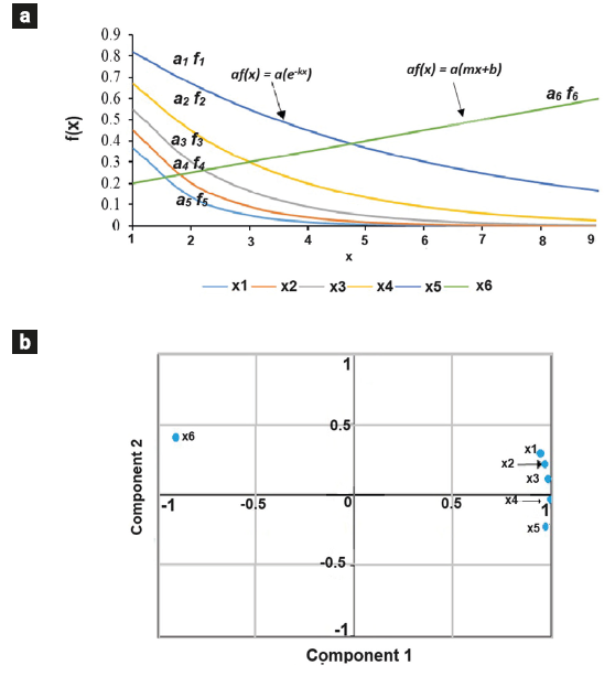
Figure 1a shows parallel lines (f(x)=mx+b) of a correlated variables system. Each line is a vector fi (x) multiplied by a scalar αi. The sum of vectors multiplied by its respective scalar gives a new vector f multiplied by a respective scalar α, which is to say, the lines are a linear combination. This new vector is the principal component and represents the linear combination of the original variables (Joliffe and Cadima, 2016). The variables of this example can be represented perfectly by the principal component (Figure 1b) due to the correlations or loading between the original variables, and the principal component is equal to 1. Similarly, in an undisturbed environment, the gradual change of air temperature in a topography area can be represented graphically as parallel lines or patterns and then by principal components. On the contrary, when a line is not parallel to the others (Figure 2a) due to the system being modified or perturbed, the variables are represented by two principal components (Figure 2b). In the first example, one principal component represents all original variables; in the second example, the representation is partitioned by two components. The use of principal components to explore patterns and perturbations is reported in the literature (Abid et al., 2018; Blommer and Rehm, 2014; Imtiaz and Sarwate, 2016; Hajrya and Mechbal, 2013). On the basis above described, we analyzed the modifications of air temperature gradient among urban, agricultural, and forest environments in the Mexican Highland.
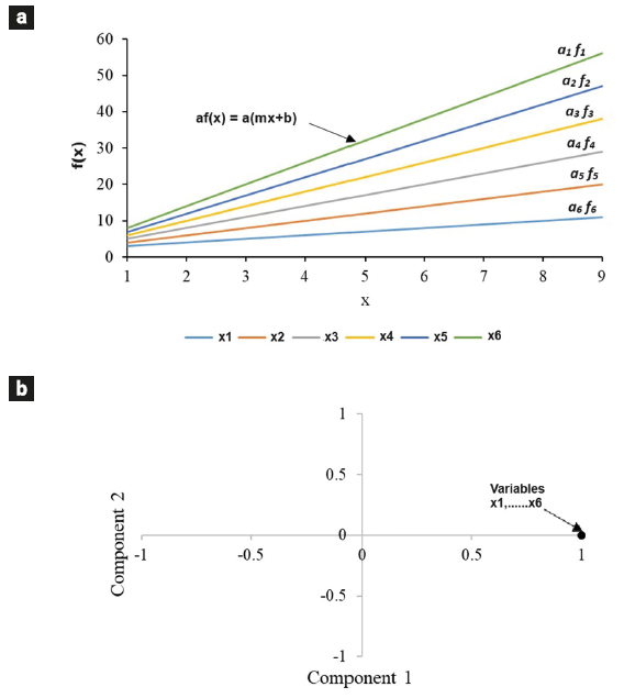
Figure 1 Parallel lines of gradually change variables (a), perfectly represented variables by component 1 (b).
2. Materials and Methods
2.1 Weather stations
Air temperature data recorded on the following weather stations from 2016 to 2019 were used: Huamantla (Hla), located in an agricultural area; Tlaxcala (Tla), located in the urban area of Tlaxcala City; La Malinche I (LMI), and La Malinche II (LMII), both located on the north and south slopes of the La Malinche stratovolcano forest, respectively (Figure 3). The data were obtained from the Mexican Meteorological Service (Servicio Meteorológico Nacional) (SMN) website (https://smn.conagua.gob.mx/es/observando-el-tiempo/estaciones-meteorologicas-automaticas-ema-s). Meteorological variables were collected and monitored at these stations based on the World Meteorological Organization (SE, 2013; Fernández et al., 2015). Regarding altitude and distance among the weather stations, the Tla and Hla have a minor altitude difference (10 m) but the most extensive distance (35.3 km). On the other hand, the Hla and LMI have the most remarkable altitude difference (709 m) but are closer (14.1 km). Table 1 shows more data about the weather stations.
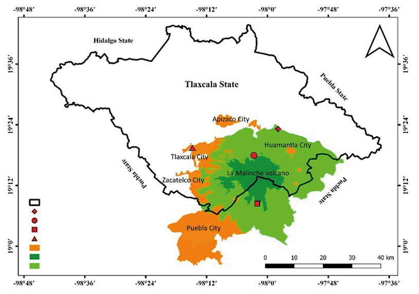
Table 1 Information on weather stations.
| Weather
Station |
Coordinates | Altitude (*masl) | Type | Environmental
condition |
|
| West Latitude | North Longitude | ||||
| Tlaxcala (Tla) | 98°14'48" | 19°19'29" | 2232 | Synoptic meteorological automatic | Urban (area of Tlaxcala City) |
| Huamantla (Hla) | 97°57'59" | 19°23'10" | 2222 | Meteorological automatic | Agricultural (area of Huamantla Valley) |
| La Malinche I (LMI) | 98°02'39" | 19°17'51" | 2931 | Meteorological automatic | Forest (northern slope of La Malinche volcano) |
| La Malinche II (LMII) | 98°01'56" | 19°08'27" | 2748 | Meteorological automatic | Forest (southern slope of La Malinche volcano) |
*masl: meters above sea level
The air temperature perturbation among urban, agricultural and forest environments was analyzed on a diurnal, daily, and monthly basis.
2.2 Diurnal air temperature analysis
The diurnal analysis was carried out using air temperature data registered every 10 minutes (T 10). It considered two diurnal intervals: the first corresponds to the warming phase from 7:30 to 14:30, and the second is the cooling phase from 15:30 to 22:30 hours local time. The warming and cooling rates were calculated for each day in both phases. These intervals were selected because the maximum air temperature peak occurs between 14:30 and 15:30 in the study area. The maximum temperature peak is reached at different day hours (Sun, 2016; Nwofor and Dike, 2010). The warming and cooling rates were estimated using the slope of the linear regression equation. Radons et al. (2019) reported better performance of a linear function than the sinusoidal function in the morning, immediately after twilight, when the temperature changes are more pronounced. The linear regression equation used is (McBean and Rovers, 1998):
Where:
air temperature every 10 minutes |
|
α= |
the ordinate at the origin |
β= |
warming or cooling rate |
t i = |
every 10 minutes |
ε i = |
random error |
A comparison of warming and cooling rates was made among the four years in a weather station (vertically shaded) and the four weather stations in a year (horizontally shaded) (Table 2). This comparison could be called orthogonal comparison. Ergo resulted in 48 comparisons, for example, Tla-16 with Tla-17, Tla-16 with Hua-16, and so on.
Table 2 Comparison among weather stations and year.
| Year | Weather station | ||||
| Tla | Hua | LMI | LMII | ## | |
| 2016 | Tla-16 | Hua-16 | LMI-16 | LMII-16 | 6 |
| 2017 | Tla-17 | Hua-17 | LMI-17 | LMII-17 | 6 |
| 2018 | Tla-18 | Hua-18 | LMI-18 | LMII-18 | 6 |
| 2019 | Tla-19 | Hua-19 | LMI-19 | LMII-19 | 6 |
| # | 6 | 6 | 6 | 6 | 48 |
# Number of comparisons among the four years in a weather station, ## Number of comparisons among the four weather stations in a year
The comparison of warming and cooling rates among the years and weather stations was made using the Kruskal-Wallis nonparametric test (McBean and Rovers, 1998):
Where:
H = |
Kruskal-Wallis statistic |
R 1,R 2,…,R 16 = |
sum of warming or cooling rates in each group formed by a weather station and a year (a cell in Table 2). |
n 1, n 2,…,n 16 = |
number of warming or cooling rates (observations) in each group (weather station-year) |
N = |
total number of warming or cooling rates in the sixteen groups |
The warming and cooling rates were analyzed in the sixteen weather station-year groups using the principal components analysis (PCA). The PCA is a mathematical procedure that transforms a system of correlated variables into another of uncorrelated variables to reduce its dimensionality and determine linear combinations (Daultrey, 1976; Schuenemeyer & Drew, 2011). As in the introduction mentioned, the principal component is the linear combination of original variables and is the new vector multiplied by a scalar or eigenvalue (λi), which in turn represents the variance of original variables. In this study, those variables are the warming or cooling rates in the groups. The variables of a system can be represented by one principal component (Figure 1a), and its eigenvalue represents 100% of the variance of the original variables. Otherwise, when the variables are represented by two or more components, the original variables' variance will not be distributed by only one eigenvalue. The eigenvalues were calculated with the characteristic equation of the matrix {R}:
Where:
{R}= |
correlation matrix of warming or cooling rates in each group |
λ i = |
eigenvalues of the principal components |
{I} = |
identity matrix |
The loads or correlations of the principal components with the warming and cooling rates in each group were calculated with the following matrix equation:
Where:
{L} = |
matrix of loads or correlations between the principal components and the warming and cooling rates in each group |
{E} = |
matrix of eigenvectors associated with each eigenvalue |
{Λ}= |
diagonal matrix of λi, the elements outside the diagonal are zero |
When the original variables are represented by a unique principal component, the loading or correlation of each variable with the principal component is perfected, that is, the element of the first column (li1) of matrix {L} are equal to 1 (Figure 1b); otherwise, all lij elements are between -1 and 1 (Figure 2b).
2.3 Daily and monthly air temperature analysis
The daily analysis was carried out by grouping the T 10 data from 00:00 to 23:50 hrs. local time. Therefore, each day had 144 values, with which the daily air temperature statistics: average (T ave,d ), maximum (T max,d ), minimum (T min,d ), standard deviation (T ave,d ), and range (T Ra,d ), were estimated for the sixteen weather station-years groups. T max,d and T min,d were selected from the 144 values. T ave,d and T SD,d were calculated using the 144 values. The calculus of T ave,d with the 144 values is more robust because the average is underestimated if it is calculated by (T max,d +T min,d )/2, due to the assumption of a symmetric rise and fall of temperature during the day (Bernhardt et al., 2018). T Ra,d was calculated subtracting T max from T min . The monthly analysis was carried out by grouping T 10 data according to the month. The monthly air temperature statistics were similar to daily statistics: average (T ave,m ), maximum (T max,m ), minimum (T min,m ), standard deviation (T SD,m ) and range (T Ra,m ). The daily air temperature statistics for the four weather stations and years were analyzed using the K-W test and PCA, just as it was in diurnal air temperature (previous section).
3. Results
3.1 Diurnal air temperature
3.1.1 warming and cooling rates
The correlation coefficients of T 10 versus time were significant (p<0.05) in all sixteen groups (4 years X 4 weather stations). The box and whisker plots of warming and cooling rates are in Figure 4. The average warming rates had an interval from 2.6×10⁻² °C·10 min-1 (in the LMI weather station and 2016 year, abbreviated as LMI-16) to 3.4×10⁻² °C·10 min-1 (Hua-19). The minimum warming rate had values from 3.1×10⁻⁴ °C·10 min-1 (LMI-16) to 6.9×10⁻³ °C·10 min-1 (Hua-19), and maximum warming rates were from 5.0×10⁻² °C·10 min-1 (LMI-16) to 8.1×10⁻² °C·10 min-1 (Hua-19). The ranges had values from 5.0×10⁻² (LMI-18) to 7.9×10⁻² °C·10 min-1 (Hua-18), and the standard deviations were from 9.6×10⁻³ °C·10 min-1 (LMI-19) to 1.5×10⁻² °C·10 min-1 (Hua-17).
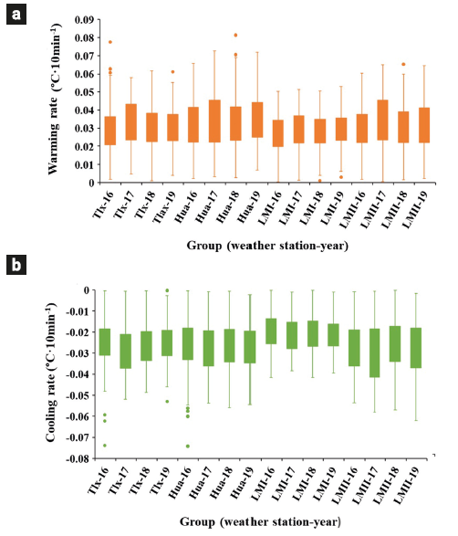
Concerning cooling rates, the average values of the groups were from -3.0×10⁻² °C·10 min-1 (LMII-17) to -2.0×10⁻² °C·10 min-1 (LMI-16). The minimum cooling rates had values from -7.4×10⁻² °C·10 min-1 (Hua-16) to -3.8×10⁻² °C·10 min-1 (LMI-17), and the maximum cooling rates were from -2.2×10⁻³ °C·10 min-1 (Hua-19) to -1.5×10⁻⁴ °C·10 min-1 (LMI-16). The cooling rates range were from 3.7×10⁻² °C·10 min-1 (LMI-17) to 7.4×10⁻² °C·10 min-1 (Hua-16), and the standard deviation values were from 7.6×10⁻³ °C·10 min-1 (LMI-19) to 1.4×10⁻² °C·10 min-1 (LMII-17).
3.1.2 Comparing heating and cooling rates
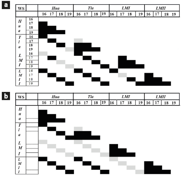
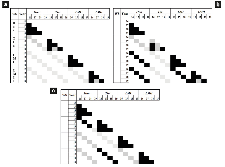
A comparison of the warming and cooling rates groups with K-W is shown in the matrix of Figure 5. The blocks indicate a group (a pair of weather station-years). The black blocks mean that a group had no significant difference (p>0.05), and the grey blocks indicate that a group had a significant difference (p<0.05). The two matrices (Figure 5a and Figure 5b) have similar distribution of the blocks. That means that in the weather station year, the warming and cooling rates are similar with the K-W test, except for the diagonals´ blocks marked by the ellipses. The diagonals show that at the Tla and LMI, and the LMI and LMII weather stations, the warming rates showed no significant differences, while the cooling rates did. The Hua and LMI weather stations significantly differed in the warming and cooling rates. The warming and cooling rates in the years in each weather station had no significant difference, except for 2016 and 2017 at the Tla weather station. In percentage terms, the matrix warming rates had (6/48)*100= 12.5% of grey blocks, while the matrix cooling rates had (13/48)*100= 27% of grey blocks, both with significant differences.
3.1.3. Principal component analysis of warming and cooling rates
The principal component analysis (PCA) showed that three components represented 84% of the accumulated total variance of warming rates in the sixteen groups (Figure 6). The eigenvalue (λi) of each component represents the total variance of the original variable. Components 1, 2, and 3 represented 59%, 18%, and 7% of the total variance, respectively. Figure 7a shows the correlations of the warming rates of the sixteen groups with the components 1 and 2. The correlation or loading between the original variables and components is given by L values (equation 4). The warming rates with component 1 had correlation values from -0.91 to -0.41, and with component 2, they had values from -0.43 to 0.84 (indicated with red lines in the figures). These correlations values formed two subgroups of weather stations based on years, one composite with 2017, 2018 and 2019, and another with 2016.
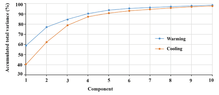
Figure 6 Accumulated total variance of principal components for air temperature warming and cooling rates.
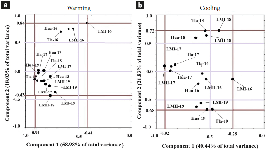
Figure 7 Warming a) and cooling b) rates correlations with two principal components for weather station-year groups.
Concerning the cooling rates, the PCA showed that 79% of the total variance was represented by three components (Figure 6). Components 1, 2 and 3, correspond to 40, 22 and 17%, respectively. The correlations between cooling rates and the component 1 were from -0.92 to -0.28, and the correlations with the component 2 were from -0.68 to 0.72. Figure 7b shows the correlations of cooling rates with components 1 and 2. It is observed that, unlike the figure of warming rates, the cooling rates form four groups composite by the weather stations according to the years. The groups of cooling rates for 2018 and 2019 have diametrically opposite correlations (positive and negative values) with component 2. The group of cooling rates for 2017 had negative correlations with component 1. The group of cooling rates for 2016 had poorly correlated with component 2.
3.2 Daily air temperature
3.2.1 Average, minimum, maximum, standard deviation, and range
The average (T ave,d ), minimum (T min,d ), maximum (T max,d ), standard deviation (T SD,d ) and range (T Ra,d ) daily air temperature, calculated with T 10 data are depicted in Figure 8. The average daily air temperature (blue line) of the Tla weather station is on top, followed by Hua (red line), LMII (pink line), and LMI (green line) weather stations (Figure 8a), this kind of behavior is shown too in the maximum daily air temperature (Figure 8b), but no like that in the case of minimum air temperature, which behavior was as follows: Tla, LMI, LMII, and Hua weather stations (Figure 8b). For the case of standard deviation and range statistics, the Hua weather station is on top, followed by Tla, LMII, and LMI weather stations (Figure 8, c, and d). The lowest and highest values and their corresponding date are in Table 3. The lowest T ave,d was calculated in Hua weather station, and the highest was calculated in Tla weather station. As to T max,d , the lowest and highest values were calculated in the LMII weather station. The lowest and highest T min,d were calculated in the same weather stations as the calculated for average. Concerning T SD,d and T Ra,d , the lowest and highest were calculated in LMII and Hua weather stations, respectively. The lowest values of these statistics occurred in winter, and the highest occurred in spring.
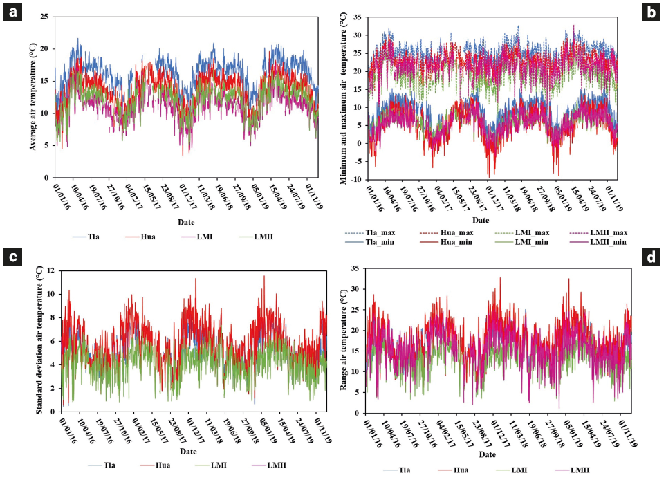
Figure 8 Daily air temperature: a) average, b) minimum and maximum, c) standard deviation, d) range.
Table 3 Lowest and highest values of air temperature statistics.
| Statistics | Lowest | Highest |
| Average daily | Hua-dec-17
Agricultural: 3.4°C |
Tla-may-16
Urban: 21.6°C |
| Maximum daily | LMII-ene-16
South-forest: 6.4°C |
LMII-abr-19
South-forest: 32.9°C |
| Minimum daily | Hua-dec-17
Agricultural: -9.4°C |
Tla-oct-17
Urban: 15.4°C |
| SD daily | LMII-nov-18
South-forest: 0.3°C |
Hua-ene-19
Agricultural: 11.5°C |
| Range daily | LMII-nov-18
South-forest: 1.1 °C |
Hua-ene-19
Agricultural: 32.4°C |
The most frequent T ave,d and T max,d were higher in the Tla weather station from 16 to 18°C and from 25 to 30°C, respectively, than in other weather stations. This weather station recorded 15 days with air temperatures higher than 30°C in 2019. On the other hand, Hua weather station registered more days with T min,d below or equal to 0°C than other weather stations. This weather station had 80 days with T min,d below 0°C in 2017, which was a higher number of days than the other three years. The most frequent T SD,d values were from 4 to 6°C in the four weather stations and years. The Hua weather station had more days, from 132 to 151, with T SD,d values from 4 to 6°C, except for 2017, in which values from 6 to 7°C in 60 days were calculated. The most frequent T Ra,d values were from 10 to 20°C at the four weather stations. In 2019, the LMI weather station had 194 days with T Ra,d values from 10 to 15°C, the highest number of days with this air temperature range.
3.2.2. Comparing daily air temperature statistics
The comparison of daily air temperature statistics of the four weather stations and the four years is presented similarly to the comparison of warming and cooling rates. The matrix comparison of the K-W test for each statistic is in Figure 9. T ave,d and T max,d had similar results (Figure 9a), as well as T SD,d and T Ra,d (Figure 9c). T min,d had a different matrix comparison (Figure 9b) compared to the other statistics. The four years in each weather station had no significant differences (black blocks) except for T min,d at the Tla weather station in 2016 and 2017. T ave,d and T max,d were significantly different among the weather stations in all years. T min,d was significantly different at the Tla weather station compared to the other three weather stations. T SD,d and T Ra,d at Tla weather stations were not significantly different compared with the Hua and the LMII weather stations. Among the other weather stations, they were. The average and maximum air temperature comparison matrix had (26/48)*100= 54.16% of grey blocks significantly different, the minimum air temperature comparison matrix had (16/48)*100= 33.3% of grey blocks. The standard deviation and range comparison matrix had (17/48)*100= 35.4% of grey blocks.
3.2.3. Principal component analysis of daily air temperature statistics
The accumulated total variance of T ave,d , T max,d , T min,d , T SD,d , and T Ra,d , represented by the principal components are shown in Figure 10. The PCA showed that three components represented about 90% of the accumulated total variance of T ave,d and T min,d statistics, while four components did it for T max,d , T SD,d , and T Ra,d . Components 1, 2, and 3 represented about 75%, 9%, and 5% of T ave,d and T min,d total variance, respectively. T SD,d , and T Ra,d had a similar representation of accumulated variance by the components, the first three components represented 79% of the accumulated total variance. Components 1, 2, and 3 represented about 44%, 23%, and 12% of the accumulated total variance of T SD,d , and T Ra,d . T max,d was represented in less measure for the first three components with a value of 77%. Components 1, 2, and 3 represented 37%, 24%, and 16% of the accumulated total variance of T max,d , respectively.
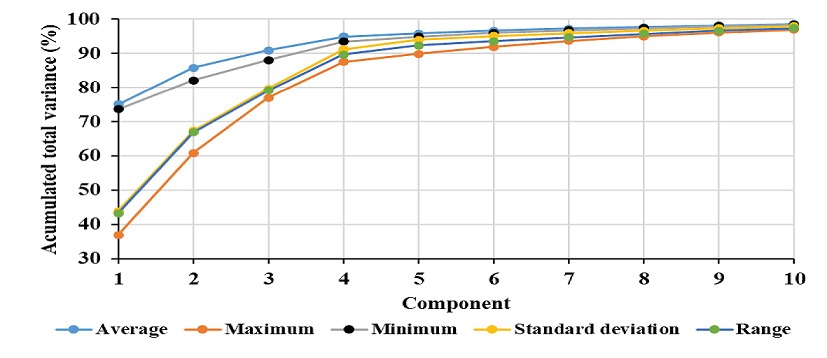
Figure 10 The accumulated total variance of principal components for daily air temperature statistics.
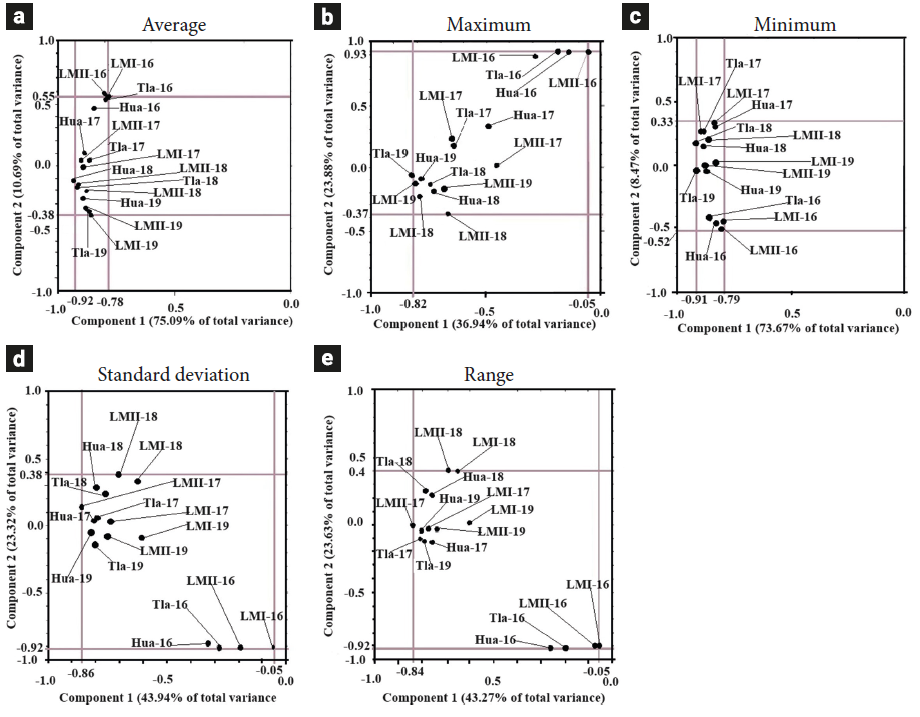
The correlations or L values (equation 4) of the sixteen weather station-year groups, with two principal components, are shown in Figure 11. It can see that the dots, which represent a weather station and a year of T ave,d and T min,d had similar dot distribution in the graph but different positions for each specific weather-year group (Figures 11a and 11c). T SD,d and T Ra,d had similar dots distribution and position (Figures 11d and 11e). The dots of T max,d (Figure 11b) differ concerning the other four statistics. The correlations between T ave,d and component 1 was around -0.78 to -0.92, and the correlations with component 2 were about -0.38 to 0.55 (red lines). T ave,d of four weather stations in 2016 formed a group because they had positive correlations of about 0.5 with component 2. The correlations between T max,d and component 1 was about -0.06 to -0.82, and the correlations with component 2 were about -0.37 to 0.93. The four weather stations in 2016 formed a group because their correlation rounded 0.9 with component 2. T min,d had correlations with component 1 from -0.91 to -0.79 and with component 2, from -0.91 to -0.79. T min,d in 2019 had the lowest correlation with component 2, while in the T ave,d analysis, the weather stations in 2017 had the lowest correlations with this component. T SD,d and T Ra,d had correlations of about -0.05 to -0.9 with component 1 and about -0.9 to 0.4 with component 2. Due to this, the weather stations of 2017, 2018, and 2019 formed a group, while the weather stations of 2016 formed another.
3.3 Monthly air temperature
The average, minimum, maximum, standard deviation, and monthly range of air temperature, calculated grouping T 10 data by month are shown in Figure 12. The highest values of the monthly average (T ave,m ) and maximum (T max,m ) were observed from April to May, and the lowest in December and January. These parameters were the lowest in the north and south forest weather stations, followed by the agricultural and urban weather stations. The lowest values of the monthly minimum (T min,m ) were in January, and the highest were from June to October. T min,m values were higher in the urban weather station and dropped in the agricultural weather station. The monthly standard deviation (T SD,m ) and range (T Ra,m ) presented upper values from November to January and lower ones from June to October. T SD,m and T Ra,m presented the lowest values in the north and south forest weather stations, and the highest values in the agricultural weather station.
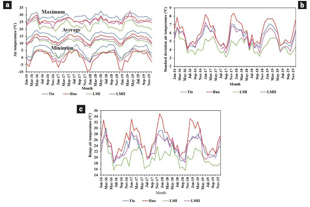
Figure 12 Monthly air temperature statistics: a) average, maximum, and minimum, b) standard deviation, c) range.
Table 4 Statistics of minimum and maximum daily air temperature.
| Weather
station |
Minimum daily air temperature | ||||||
| n | Ave | Min | Max | Kurtosis | Skewness | S. D. | |
| Tla | 1212 | 8.9 | -2.8 | 15.4 | -0.28 | -0.60 | 3.33 |
| Hua | 1398 | 5.2 | -9.4 | 13.6 | -0.20 | -0.40 | 4.15 |
| LMI | 1329 | 5.7 | -1.4 | 11.9 | -0.25 | -0.45 | 2.34 |
| LMII | 1265 | 5.6 | -3.5 | 12.0 | -0.20 | -0.42 | 2.84 |
| Weather
station |
Maximum daily air temperature | ||||||
| n | Ave | Min | Max | Kurtosis | Skewness | S. D. | |
| Tla | 1212 | 25.4 | 10.7 | 32.7 | 1.97 | -0.70 | 2.73 |
| Hua | 1398 | 22.8 | 8.5 | 30.0 | 1.44 | -0.58 | 2.68 |
| LMI | 1329 | 18.8 | 7.2 | 28.1 | 0.16 | -0.08 | 3.15 |
| LMII | 1265 | 21.2 | 8.3 | 32.9 | 1.46 | -0.48 | 2.84 |
Figure 12 shows that T ave,m , T max,m , and T min,m had an increasing stage from January to May, a flat line from June to July, and a decreasing stage from August to December. The T SD,m and T Ra,m behaviors were opposite to T ave,m , T max,m , and T min,m . In the phases from January to May and from August to December, the inter-monthly changes of T ave,m and T min,m were more noticeable than T max,m , T SD,m and T Ra,m . In the January to May phase, T ave,m , T max,m and T min,m showed positive and T SD,m and T Ra,m negative slopes, with values of 1.5, 1.2, 1.9, -0.2, and -0.8 °C/month, respectively. From August to December, the changes were the opposite, with negative slopes of T ave,m , T max,m and T min,m and positive for T SD,m and T Ra,m , with values of -1.0, -0.2, -1.7, 0.47, and 1.5°C/month, respectively.
4. Discussion
4.1 Diurnal air temperature
4.1.1 warming and cooling rates
The statistics analyzed (average, minimum, maximum, and range) had different values between warming and cooling rates in the sixteen groups (Figure 5), except for standard deviation, which had values rounded to 1.0×10⁻² °C·10 min-1 in both types of rates. The average warming and cooling rates fluctuated similarly between groups, but with opposite sign rounding 3.0×10⁻² °C·10 min-1 for warming rates and -3.0×10⁻² °C·10 min-1 for cooling rates. The minimum rates had more fluctuation between the groups in the cooling phase than in the warming phase. The highest minimum values of cooling rates are in the forest (LMI weather station) and the lowest in urban (Tla weather station in 2016) and agriculture (Hua weather station in 2016), it may be because 2016 was an El Niño year (Martínez et al., 2017). In contrast to the minimum, the maximum had more fluctuation in the warming phase than in the cooling phase. However, the lowest values of maximum warming rates are in forests and the highest in agriculture and urban weather stations. The range of warming rates was dissimilar to the range of cooling rates. These results show that the vegetation of the forests dampens the air warming by biophysical mechanisms (Li et al., 2015) and by the suppression of mixing due to the lower roughness of the open areas, which causes the temperatures to rise more rapidly than in the forests (Lee et al., 2011). However, these differences between the forest and the agricultural area can also be caused by elevation in sites (Good, 2015; Hemond and Fechner, 2015).
4.1.2 Comparing heating and cooling rates
Multiple comparisons of warming rates between the weather stations-years combinations, with the K-W test, and comparisons of cooling rates showed that environmental conditions heat up at similar rates in 87.5% of combinations and cool down in 73%. The consistent warming rates differences between agricultural (Hua weather station) and forest of the north side of La Malinche volcano (LMI weather station) in 2016, 2018, and 2019 stand out. The cooling rates significantly differed between the agricultural, urban, and forest areas of the north side of La Malinche volcano and between the north and south forests of La Malinche volcano (Figure 4b). The forest cooling rates of the north slope of La Malinche volcano (LMI weather station) are higher than the south forest (LMII weather station). The differential cooling rates in La Malinche volcano can be due to its symmetrical conical shape, its location in the north latitude, and that it is an isolated volcano in the trans-Mexican volcanic belt (Castro-Govea and Siebe, 2007), all of them causing that the north side is less exposed to the sun. Nevertheless, the cooling rate of the forest's south slope is comparable to the agricultural and urban areas.
4.1.3 Principal component analysis of warming and cooling rates
The PCA showed that three components represented the total variances of the warming and cooling rates, rounding 80%. This percentage was comparable to those reported in the analysis of other climatological variables (Bethere et al., 2017; Isaak et al., 2018; Zuśka et al., 2019). In general, this indicated that warming and cooling rates in the sixteen groups of weather stations-years meet the criteria that the groups can be a linear combination (Schuenemeyer and Drew, 2011) or covariate similarly (Hurth and Pokorna, 2005). However, the variance values components indicate that air temperature warming rates were partially a linear combination forming two groups among years, one for 2017, 2018, and 2019 and another for 2016. This result indicates a perturbation relating air temperature among the urban, agricultural, and forest environments studied. Concerning cooling rates, the linear combination was weaker; in other words, there was more perturbation because the variance representativeness of component 1 was equal to 40%. In this case, the dots representing weather stations-year were more disperse, according to Figures 7a and 7b. The dots distribution in Figures 7a and 7b also indicates that the air temperature warming rates are different from cooling rates. This clearly shows the effect of forest, agriculture, and urbanization. If variation in air temperature were due to the altitudinal and spatial gradient, then the dots would be concentrated in some place on the graphic and would be a perfectly linear combination with rounding values of 100% by the first principal component. Consequently, the PCA could be a valuable tool to detect changes in air temperature gradient caused by perturbation of the system.
4.2 Daily air temperature
4.2.1 Average, minimum, maximum, standard deviation, and range
The analysis of air temperature statistics showed that the lines of the average and the maximum urban weather station were on top in the graphics, followed by agricultural, south forest, and north forest of La Malinche volcano. The minimum air temperature had behavior where the urban weather station was on top, followed by south forest, north forest, and agricultural weather stations. The standard deviation and range were similar to the average and the maximum, but agriculture had the highest values, followed by urban and forest weather stations. The average, maximum, standard deviation, and range in the forest were lower than in agricultural and urban areas. The average and maximum difference is due to altitude (Hemond and Fechner, 2015; Chen et al., 2018; Isaak et al., 2018), which between forest and urban and agricultural weather stations is from 500 to 700m (Table 1). However, the differences in daily temperature between urban and agricultural areas cannot be attributed to the effect of altitude since there is a difference of 10 meters between them. The lower values of standard deviation and range in the forest are possibly due to the vegetation cover. The literature describes that forests have an important but complex role in air temperature (Li et al., 2015; Lee et al., 2011; Shiflett et al., 2017; De Frenne et al., 2019). The minimum air temperature values in the forest were between urban and agricultural, which means that the forest buffers air temperature.
The T ave,d and T max,d most frequent values were higher in the urban environment than in agricultural and forest. That could be because, in urban areas, the air temperature increases with its size compared to its surroundings (Zhuo et al., 2017). The T max,d >30°C occurs when a heatwave is presented (Rosenzweig et al., 2006). A heatwave was registered throughout the country in 2019, which caused the air temperature rise above 30°C (Pascual et al., 2019) in the urban areas but not in forest and agricultural ones.
The T min,d most frequent values in the urban area were higher than in the agricultural and forest areas. In the agricultural area, devoid of vegetation in winter, the highest number of days with temperatures below 0°C, caused by cold fronts, were recorded (Pascual et al., 2019). The urban area had fewer days, with T min,d <0°C and more days with T max,d > 30°C. In agricultural areas, there were more days with T min,d <0°C, than in urban and forest areas. This result clearly shows that the forests buffer the ambient temperature because they did not show T min,d <0°C in the agricultural area nor T max,d > 30°C in the urban area.
The most frequent values of T SD,d and T Ra,d in the agricultural area were higher than in urban and forest areas, accentuating the T Ra,d difference between the agricultural and forest areas because the vegetation cover reduces the range temperature (Lee et al., 2011). In winter, T Ra,d was higher than in summer-autumn in the three environmental conditions; this result is comparable to that reported in the literature (Qu et al., 2014). In winter, T Ra,d is higher due to the lack of cloudiness (Braganza et al., 2004; Roy and Balling Jr., 2005), cold fronts (Pascual et al., 2019), and the lack of vegetation cover (Lee et al., 2011), which cause more significant fluctuations in temperature during the day.
4.2.2 Comparing daily air temperature statistics
According to the environmental conditions analyzed, we expected that the air temperature differences could be among urban, agricultural, and forest, but not among years. Indeed, regarding the latter, the K-W test showed that among years, there were no significant differences, except for minimum air temperature at urban conditions. The K-W test showed that the environment conditions analyzed were significantly different (p<0.05) based on Tave,d and Tmax,d. With Tmin,d, TSD,d and TRa,d, the differences between the environmental conditions were not consistent. It is plausible to say that the temperature differences between urban and agricultural areas are not due to altitude because both have a difference of 10 m, but according to their environmental conditions and the differences between the north forest and the south forest are due to position in the La Malinche volcano. The north forest is located at a higher altitude and is less exposed to solar radiation compared to the south forest, which is located at a lower altitude and is more exposed to solar radiation.
4.2.3 Principal component analysis of daily air temperature statistics
The PCA showed that the total variances of T ave,d and T min,d were represented (>80%) by two components, while T max,d , T SD,d and T Ra,d , by three components. Similarly to warming and cooling rates, the analysis using five statistics indicated that daily air temperature can be a linear combination (Schuenemeyer and Drew, 2011; Hurth and Pokorna, 2005) but with a perturbation degree characterized by the variance of components. The correlation values (Figure 10) showed that the linear combination of the environmental conditions is based on years. The statistics (T max , and T Ra,d ) for 2016 resulted in a partially linear combination, and those for 2017, 2018, and 2019 resulted in another. This result reveals that although the thermal gradient is still preserved in the study area, if the urbanization and the agricultural regions continue increasing, and so does the reduction of the forest, the natural thermal gradient is at risk of breaking. The conjugation of the results of the K-W test and the PCA showed that the temperatures had significant differences and were a partially linear or perturbed combination.
4.3 Monthly air temperature
The monthly behavior of T ave,m , T max,m and T min,m showed that the values were higher in April and May and lower in winter. This is probably due to the minimization of topographic factors during the winter months, the short duration of the day, and the lowest angle at which the sun's rays strike the earth's surface (Dutta et al., 2017). In the agricultural area, the inter-monthly changes of T ave,m , T min,m , T SD,m and T Ra,m , were more significant than in the forest and the urban area. This result is comparable to that reported in the literature (Shiflett et al., 2017; Rushayati et al., 2018; Wong and Peck, 2005). The inverse behavior of T SD,m and T Ra,m concerning T ave,m , T max,m and T min,m , shows the effect of rainfall and cold fronts in the study area from May to June and November to February, respectively.
The T ave,m in the agricultural and forest areas was lower than average monthly air temperature (1981-2010), while in the urban areas, they were higher in March, April, October, November, and December 2019. In these months, Pascual et al. (2019) reported similar monthly temperatures on a national scale (Mexico). Concerning the monthly T max,m , they were lower than their respective normal ones in the three environmental conditions. There weren't significant differences between the T max,m and normal ones in the agricultural area, while the most considerable difference was in the forest.
In the three environmental conditions, the monthly T min,m was higher than the average minimum air temperature. Monthly T min,m increasing was more accentuated in urban areas than in agriculture and forest areas. The T min,m increased more than the monthly T max,m ; this result is consistent with that reported in other studies (Qu et al., 2014; Machiwal et al., 2019). From January to May, the monthly changes of T ave,m , T max,m and T min,m were lower than those reported by Chinchorkar et al. (2013), but the changes from August to December were more significant than those of the same authors. The monthly changes of T min,m were comparable to those reported in the literature (López-Díaz et al., 2013; Colunga et al., 2015).
5. Conclusions
The five statistics (average, minimum, maximum, standard deviation, and range) had no values persistent in warming and cooling rates. The K-W test showed that warming and cooling rates are significantly different between the agricultural, urban, and forest areas. Even the north and south sides of La Malinche volcano have a significant difference in cooling rate. The PCA showed that the warming and cooling rates were partially a linear combination in the agricultural, urban, and forest. Still, cooling rates had less value of variance, indicating a high degree of perturbation in these environmental conditions. In others words the cooling rate is more sensitive to show the system perturbation.
The average, maximum, and minimum air temperature in urban, standard deviation, and range in agriculture had the highest values in graphics. These differences between urban and agricultural environments cannot be attributable to altitude but to cover vegetation and topography
Comparing air temperature along years, there were no significant differences except for minimum air temperature in the urban environment. The average and maximum daily air temperatures significantly differed between the environmental conditions. The daily air temperature on the north side of La Malinche resulted in a significant difference concerning the south side, likely due to solar radiation incidence.
The maximum, standard deviation, and range daily air temperature in urban, agricultural, and forest environments showed more perturbation degrees than average and minimum air temperature. The statistics of air temperatures showed significant differences in the environments, and the PCA showed that they are perturbed.
The monthly behavior of average, maximum, and minimum air temperature showed that the values were higher in April and May and lowered in winter; standard deviation and range had inverse behavior. The average monthly air temperature in the agricultural and forest areas was lower than the normal monthly air temperature (1981-2010). While in the urban area, they were higher in March, April, October, November, and December. The monthly minimum air temperature increase was more accentuated in urban areas than in agriculture and forest areas, and the minimum increased more than the maximum monthly.

