




 nueva página del texto (beta)
 Inglés (pdf)
 Artículo en XML
 Referencias del artículo

 Traducción automática
 Enviar artículo por email
 Citado por SciELO
 Similares en
SciELO

 Permalink


1. Introduction
Among the most harmful natural phenomena for mankind are earthquakes. One way to mitigate those damages is through prevention. Building regulations have precisely that function. For the elaboration of a realistic regulation for a certain locality, the observations of local damages occurred during earthquakes must be taken into account or, in the other hand, measurements of the mechanical characteristics of the soil in different parts of the city. The distribution of damage during large earthquakes often depends on so-called site effects. Subsurface impedance contrasts can significantly amplify the ground motion, as well as increase ground motion duration. Mapping of places with site effect also called microzoning, has been carried out in large cities around the world (Pergalani et al, 2020, Keil et al. 2020, Zalbuin et al, 2021). A large number of these types of studies have relied on ambient vibration records given the ease and low cost with which the data can be obtained. Seismic noise is also used to measure the structural health of buildings in the face of possible loss of rigidity due to the occurrence of earthquakes by measuring changes in its natural frequency of vibration and amplitude (Godinez K., 2022, Vargas-Luque & Del Carpio, 2021). In early studies, site resonance frequency was deduced from spectral proportions of seismic noise records (Kagami et al., 1986; Seo, 1992), or taken as the peak frequency of the horizontal component Fourier amplitude spectrum (Kobayashi et al., 1986; Gutierrez and Singh, 1992). More recently, what has been used are the spectral ratios calculated between horizontal components relative to the simultaneously recorded vertical component (HVSR, Nakamura, 1989; Lermo and Chavez-Garcıa, 1994; Field and Jacob, 1995, among many others). It is now recognized that the HVSR technique generally provides a reliable estimate of the resonant frequency.
When we observe an amplification due to a large impedance contrast between a soft soil layer and the basement, the use of HVSR is clearly reliable (Chavez et al, 2007). A more complex local geology, however, raises the question of its reliability. It is important to understand the limitations of such a technique.
The goal of this work is to present a dynamic characterization of the city of Culiacán using the HVSR technique, reinforcing it with direct observations obtained from soil mechanics studies and multichannel analysis carried out in different points of the city.
It is important to recall the need of updating the local building regulation, attaching information related to the dynamic behavior of the soil along with stratigraphy when possible.
2. Background
2.1 Regional tectonics
Gulf of California, in front of which the state of Sinaloa is located, is a divergent boundary between the North American and Pacific plates. This boundary consists of a series of transform faults and small dispersion centers creating ridges and basins along the entire gulf and ending in the south, at the East Pacific Ridge (EPR) that marks the boundary of the Rivera plate (Fenby and Gastil, 1991; Nagy and Stock, 2000, Figure 1).
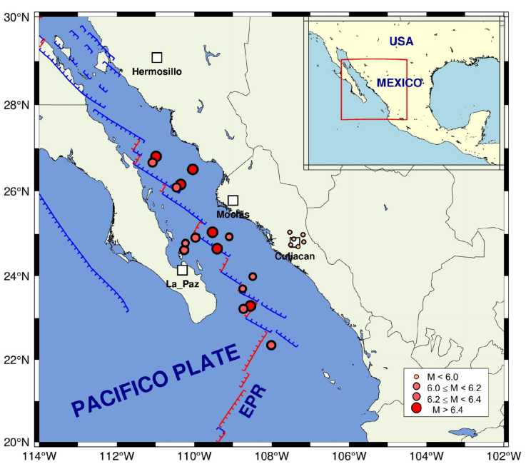
Figure 1 Regional tectonics of the area of study. Circles are epicenters. Main cities are represented by squares
Displacement speed of one tectonic plate with respect to the other in this region is estimated to be between 41 and 54 millimeters per year (Plattner et al., 2007). The southern region of the Gulf of California is an area of high seismicity. Most of the earthquakes that are generated there, are mainly related to the transform faults of right lateral behavior.
Culiacán region, has experienced the effects of earthquakes. Sixteen earthquakes with Mw≥ 6 have occurred in Gulf of California in front of Sinaloa State since 1980. The strongest, occurred on November 13, 2015 (Mw=6.6), and its epicenter was located 216 km northwest of Culiacán.
There are some active faults in the region of hills and foot-hills, parallel to the coastline that have caused low magnitude earthquakes (SSN, 2023; SGM, 1999). According to SSN catalog, at least six small events within a radius of 30 km from the city have occurred in the last 40 years. The most recently, on August 12, 2021 (Mw=3.8, Figure 1).
2.2 Geology
Mountain ranges at the east of the city consist of volcanic rocks, essentially of rhyolitic composition. Some settlements begin to occur on the slopes of these hills that rise at more than 300 m altitude. The Cerro El Tule, southeast of the city is formed from volcanic rocks of basaltic composition of Pleistocene age. It represents the last manifestation of volcanism in the region.
Most of the urban area of the city of Culiacán is settled on fluvioaluvial and lacustrine materials of very recent ages. They are composed of clastic elements of various sizes, well rounded, of diverse composition, packed in an incipiently cemented sandy matrix where small and thin levels of medium-grained sands are occasionally interspersed. They are massive sediments, with no visible stratification nor faulting, at least apparently.
Southern and NE areas of the city are settled on a sequence of conglomerates and sandstones, compact well consolidated, paleogene, reddish coloration. The most recent urban developments are based on these materials.
Towards the NE and SE of Culiacán city, spills of lavas of andesitic composition of neogene age can be observed. They are compact rocks, although fractured and partially altered, which constitute consolidated flat terrain (SGM, 1999).
The Tamazula and Humaya rivers that converge in the city of Culiacán and later from the Culiacán River, have produced diverse deposits along their courses and floodplains. These materials constitute a very particular area of clastic materials (gravel, sand, silt and clay) that constitute unconsolidated and saturated terrains (Figure 2).
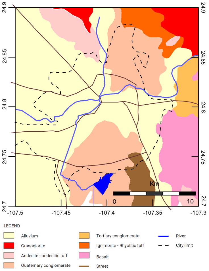
Figure 2 Geological map of the Culiacán (Modified after SGM, 1999). Dotted line indicates the boundary of the urban sprawl. The brown lines represent the most important avenues across the city.
Buildings of heights exceeding 40 m have been recently built in areas adjacent to the aforementioned rivers, which makes site effects studies, have an importance from an engineering and a civil protection point of view.
3. Analysis and results
3.1 HVSR method
Spectral ratios of horizontal components relative to the vertical recorded simultaneously have been widely used to determine site response from ambient-vibration records. The records of 113 sites within the urban area of Culiacán (triangles in Fig. 3) were analyzed. A Kinemetrics ETNA recorder with triaxial accelerometers and a sampling rate of 100 samples per second was used.
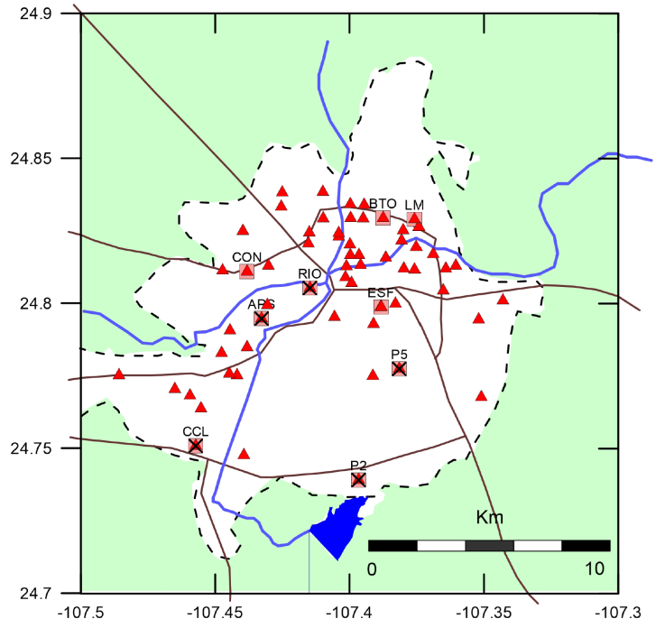
Figure 3 Location of HVSR measuring points (triangles). The white zone represents the urban sprawl of the city. Main streets and rivers are shown. Labeled squares indicate the sites where multi-channel measurements were made and velocity profiles were obtained. Crosses indicate places for which soil mechanics information is available.
At each site we obtained two or more ambient vibration records with durations of 1 to 3 minutes. In each record, we selected a window which showed the fewest transient signals and the noise appeared more stationary. We calculate the spectral relationship between horizontal and vertical movement from the selected window. These relationships produced HVSR graphs where a peak could be clearly be identified from which a dominant period value and maximum amplification was determined. Geopsy (Geophysical Signal Database for Noise array Processing) software (Wathelet et al, 2020) was used for this analysis. Figure 4 shows an example of a 3 components record, the used window and their respective HVSR with a clear peak.
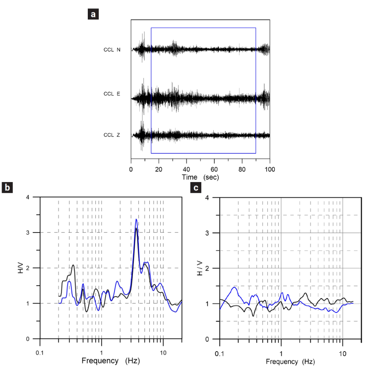
Figure 4 Example of a 3-component record a). The box in the traces indicates the window used for analysis. b) H/V spectrum with a clear peak. c) H/V spectrum where no significant peak was observed. Blue and black curves are the different estimates of H/V from different records at each site.
From the 113 records, only 61 produced HVSR with clear peaks from which a value of dominant period and maximum amplification could be determined. We attribute these results to the physical conditions when each measure was taken as they are not grouped in specific areas.
Once the dominant periods for all the 61 points were estimated, they were used to build a contour map using the Kriging spatial inference method in the context of surface geology as shown in Figure 5. The city boundary is also shown, as well as the main streets and rivers.
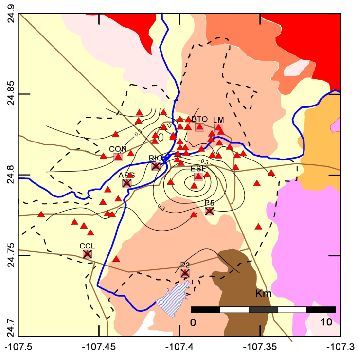
Figure 5 Contour map of dominant periods for Culiacán city. The dotted line indicates the boundary of urban sprawl.
A correlation between the dominant periods distribution and the surface geology can be observed. The alluvial zone has periods between 0.2 and 0.7 and decreases in transitions to another type of soil. Conglomerates to the northeast and south, andesite to the northwest and andesite and conglomerates to the east.
Figure 6, on the other hand, shows the amplitude distribution
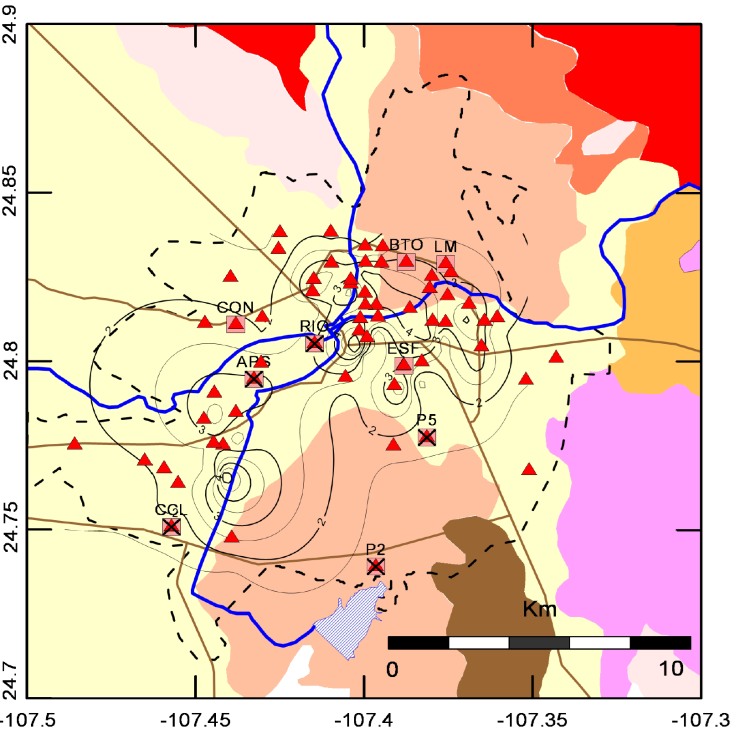
Figure 6 Contour map of amplitudes for Culiacán city. The dotted line indicates the boundary of urban sprawl.
Amplitudes between 2 and 4 can be observed. The maximum found, are located along the riverbed, in the transition zone from conglomerate deposits to alluvium.
3.2 Multichannel Analysis of Surface Waves
3.2.1 Microtremor Array Method (MAM)
In order to reinforce observations made with the HVSR technique, multichannel measurements were made at some points, velocity profiles were obtained and transfer functions calculated by means of a multichannel analysis of surface waves. Specifically using the microtremor Array Method (MAM).
Ambient vibration recorded at a measuring point is produced by different sources which arrive from different directions which makes the vibration field essentially a random field. If we correlate records from different points, we can observe a wave travelling through the surface. A surface wave.
The principle underlying the Multichannel Analysis of Surface Waves method is the dispersive nature of Rayleigh waves when they travel in a stratified medium. Different frequencies travel at different speeds. By calculating phase velocities at different wavelengths (frequencies), we can build a dispersion curve (Park et al, 1999). For an array of sensors, phase velocities are obtained by comparing the amplitude spectra of each pair of sensors.
With this multichannel approach, an image is constructed where the dispersion trend is identified from the energy accumulation pattern. The dispersion curve is extracted following the trends in the image.
We carried out measurements at nine locations throughout the city (shown as squares in Fig. 3, coinciding with single-station measurements sites). We used a PASI GEA24 exploration seismograph with a 24-bit dynamic range and a line of 24, vertical-component, 4 Hz natural frequency geophones. The sampling rate was 8 msec. This system had a flat response for velocity between 4.5 and 250 Hz. At each location, the geophones were installed with a 5-m distance between them, giving a total length of 120 m, and five time windows of about 60 sec of ambient vibration were recorded. Data is recorded in seg2 format so it can be directly read by the seisimager analysis software (test version).
The process begins with the transformation of all the records of the array, from the time-space domain (t-x), to the frequency-wave number domain (F-K) and from there, to the frequency-phase velocity domain (F-C) from which the dispersion curve of the maximum energy accumulation is obtained as shown in Figure 7.
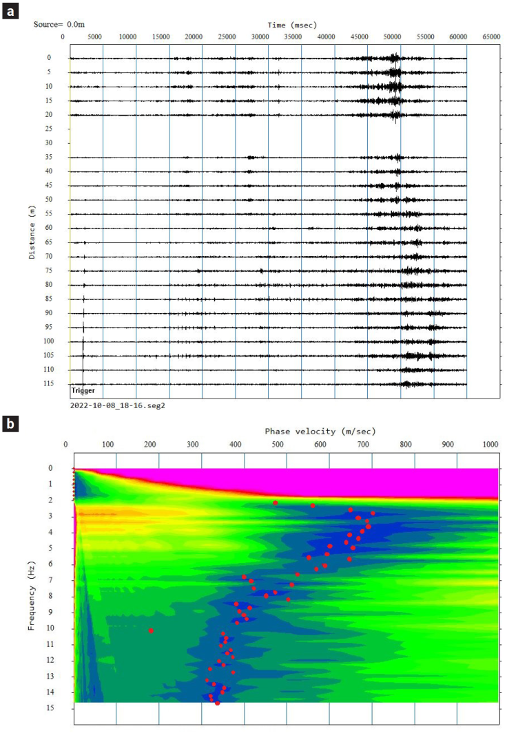
Figure 7 a) Seismic traces stacked from 4 recording windows for the RIO site. b) Estimated phase-frequency image. Red circles indicate maximum energy accumulation.
Surficial stratigraphy in terms of velocities can be estimated from the inversion of the dispersion curve by applying some standard algorithm, for example Herrmann's algorithm in which, the nonlinear inversion is replaced by a stochastic least squares procedure in which successive iterations are made until the differences between the theoretical dispersion curve obtained from the iterated model and the observed dispersion curve is small enough (Herrmann, 1973, Figure 8).
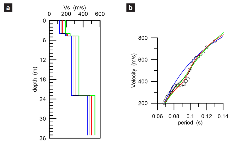
Figure 8 a) Velocity models obtained from the iterated dispersion curves. b) Iterated dispersion curves. Circles indicate the observed dispersion curve. Analysis correspond to CCL site.
For the determination of dispersion curves, the seisimager software was used. Velocity models were obtained with the Computer Programs in Seismology Software (Herrmann & Ammon, 2002).
Frequency range that could be observed in the dispersion maps, from which the dispersion curves were obtained, indicate that the velocity profiles are reliable up to 30 to 40 m depths. We compared some the obtained profiles with direct measurements of soil mechanics carried out in other specific studies. Three of them could be corroborated up to 20 m depth, one up to 30 m and one profile only up to 10 m. (Figure 9).
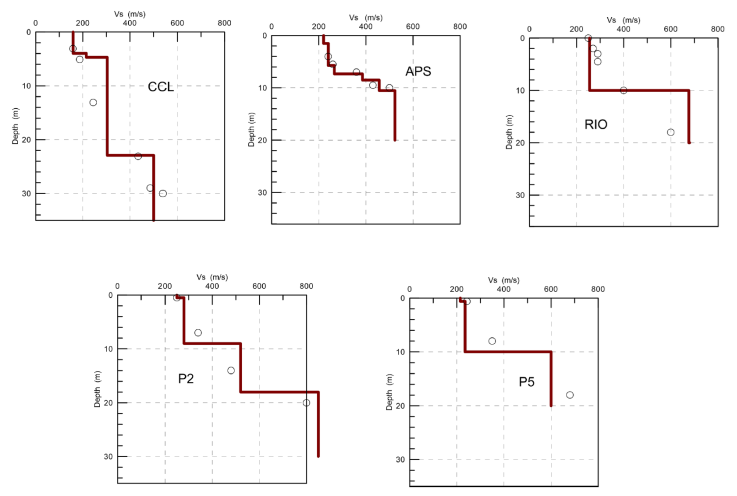
Figure 9 S-wave velocity profiles for five locations for which soil mechanics studies were available. The circles indicate the values obtained in those studies. The solid lines show the profile obtained from the inversion of the phase velocity dispersion curves observed at the corresponding location.
Direct comparison shows good agreement in all the cases which gives us confidence in the profiles obtained from the inversion process. It can be observed that the velocities in the first 8 meters are similar at all locations but from 12 to 18 meters, higher velocities can be observed at RIO and P5 locations compared with the other which suggests harder strata at these depths below these locations. P2 shows the higher velocity below 20 m. probably related to the nearby basalt deposit.
Shear-wave velocity profiles for the topmost 30 m for all nine sites are shown in Figure 10.
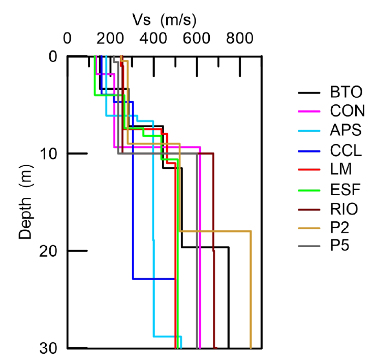
Figure 10 Shear-wave velocity profiles inverted from phase-velocity dispersion curves for the nine sites.
We can observe that the behavior of all profiles is similar up to approximately 8 m. The highest surface velocities can be seen in the P2 site which is located over conglomerate deposits, and the smallest at ESF site, located on alluvial soil. Between 10 and 20 m the lowest velocity is seen in CCL site which is a site over alluvium, farthest from the deposits of harder or consolidated material. In contrast, the highest speeds below 20 m are seen at BTO and P2 sites, reflecting the conglomerate deposits below these sites. In general, we can observe a correlation between the obtained velocities and the surface geology. Lower velocities in sites over alluvial soils, higher velocities in sites over harder deposits (conglomerate).
3.3 Transfer Functions
For modeling purposes, the site effect caused by a soil structure can be considered as the result of the convolution of energy (eg. seismic energy), which travels through a stratigraphic structure, and the site's own response called the transfer function. If the soil characteristics are known (the stratigraphic structure), the transfer function of the site can be estimated, and a total theoretical response can be obtained given any input signal by propagating it (Green's function) through the medium.
There are several ways to describe a medium based on its elastic properties: homogeneous medium, stratified medium, heterogeneous medium, etc. In this study we describe the medium as stratified with horizontal flat layers, characterized by its thickness, density, shear modulus and damping factor.
We computed the Transfer Function using two different tools to compare results. The Degtra software (Ordaz, 1988) and the SHAKE2000 (Ordoñez, 2012). Both use the transfer matrix originally proposed by Thompson (1950) and corrected by Haskell (1953). We used the corresponding shear-wave profile for each site. For the most superficial layers a damping factor of 5% was considered and for the intermediate and deep layers we use a value of 4%. Density in each layer was considered to be 1800 kg/m3. Both tools gave similar results. Figure 11 illustrates the transfer functions obtained for the 9 sites.
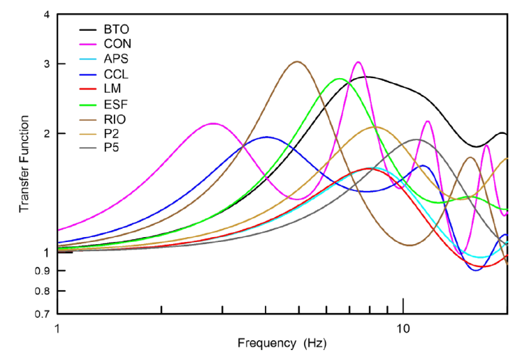
Transfer functions obtained show maximum amplifications less than or equal to 3 and fundamental frequencies between 4 and 9 Hz (0.1 to 0.25 seconds) in good agreement with dominant periods obtain by HVSR method. The greatest contribution of energy corresponds to the fundamental mode of vibration.
4. Conclusions
A dynamic characterization for the soil of Culiacán, Mexico, using the HVSR technique was performed. The results show good agreement of dominant periods with the geology shown in Figure 2. Dominant periods between 0.2 to 0.7 for the alluvial zone in the central and western part of the city and lower periods for sites near igneous rock outcrops south and southeast of the city. A multichannel analysis was carried out at 7 sites where the measurement of H / V was performed using the MAM method. The phase-velocity dispersion curves were inverted and reliable speed profiles up to 30 m were obtained. Five of them could be compared with soil mechanics data. The direct comparison in all 5 cases shows agreement. Transfer functions were computed and the dominant period values obtained with the HVSR technique were similar.
Finally, direct observations such as those obtained in this study, are essential for an adequate dynamic characterization of the soil of the city of Culiacán, Sinaloa and a very important factor to consider for a future update of the building regulations of the city of Culiacán.

