


 nueva página del texto (beta)
 Inglés (pdf)
 Artículo en XML
 Referencias del artículo
 Enviar artículo por email
 Citado por SciELO
  Similares en
SciELO
Similares en
SciELO 
 Permalink
1. Introduction
Rock characterization based on elastic responses that consider mineralogical composition and pore-filling fluids at the core, well, and field scales have been reported by rich literature on rock physics applied to earth models (Goodway and Pérez 2010, Meléndez and Schmitt 2013, Perez and Mafurt 2014, Nicolás-López and Valdiviezo-Mijangos 2016, Carcione and Avseth, 2015, Sayar and Torres-Verdín 2017, Holt and Westwood, 2016, Nicolás-López et al., 2019, and Nicolás-López et al., 2020). However, most of these reported applications are related to petroelastic models constructed from classical static Gassmann models or dynamic micromechanical models for lithology interpretation and reservoir delineation.
The petroelastic models can be defined as a connection between reservoir properties and seismic attributes of the subsurface structures. This connection is used to link seismic parameters such as acoustic and shear impedances (Ip & Is) with rock's elastic parameters as shear modulus (μ), Lamé parameter (λ), Young's Modulus (E), and Poisson's ratio (v) (Danaei et al., 2020). A well-known methodology for interpreting the amplitudes from pre-stacked seismic reflection data to produce a probabilistic distribution of subsurface lithology and pore fluid information is described in Avseth et al. (2005). As part of this sort of contribution, in which relationships between seismic and elastic parameters are noted, the job of Danaei et al. (2020) has established a connection between petroelastic information and 4D seismic information. It was carried out to optimize volumes to identify pore pressure and fluid saturation variations. Similarly, Uhlemann et al. (2016) correlated the seismic velocities with seismic tomography to highlight the importance of the modulus of elasticity (M) for a better characterization in identifying potential hydrocarbon zones with seismic images of high resolution. Bredesen et al. (2021) demonstrated how to perform a quantitative reservoir characterization using rock physics models on seismic inversion data, achieving consistent predictions of a gas-condensate reservoir.
In the present study, we also worked with rock's elastic parameters, e.g., the modulus of elasticity, lambda-rho, or mu-rho, with the difference that a micromechanical quantitative method was used. This investigation focused on identifying potential prospective hydrocarbon reservoir zones through the lithological interpretation workflow via computing elastic properties from well-logs and seismic volumes. The objective was to establish the coupled relationship that exists between the elastic parameters at well and seismic scales to determine the lithological configuration of a study area, thus simplifying the scaling process and the prediction and identification of lithologies and areas of oil interest (reservoir) making possible the scaling of any elastic parameter in 3D seismic inversion data.
The novel methodology using a micromechanical model proposed here makes it possible to identify lithologies and prospective hydrocarbon zones. It also includes a new feature: 1D-3D brittleness workflows for identifying the reservoir zones. Both petroelastic and brittleness workflows were applied to identify a reservoir in the Lower Cretaceous associated with the Stybarrow field through quantitative (hard) results (BA≥0.5). The results were consistent with those reported using other methodologies (Ementon et al., 2004; Arevalo-López 2017). Therefore, the proposed methodology represents an alternative to identifying potential oil or gas zones.
1.1. Geology setting: Barrow subbasin
The field information consists of geophysical logs and seismic information from a study area in deep water to the NW of Australia knowns as the Carnarvon Basin (Figure 1), which is a marine oil and gas-producing basin containing up to 10 km thicknesses of predominantly Mesozoic deltaic siliciclastics (Ementon et al., 2004).
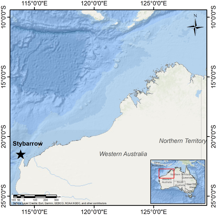
The Barrow Sub-basin is geologically an elongated marine basin trending NNE to SSW, which forms part of the North Carnarvon Basin in Northwest Australia. The Barrow Sub-basin is a deep syncline graben that forms a depocentre of about 10 km of predominantly Mesozoic and Cenozoic sequences, which are flanked to the east and west by shallow faulted terraces containing more than 5 km of Paleozoic strata from Cenozoic (Ementon et al., 2004).
The development of the basin began in the Paleozoic, generating structural changes due to intense opening processes during the Late Triassic to Early Jurassic that occurred between Australia and the Burma Block to the West of India. During the Late Triassic to Early Jurassic, deltaic sand reservoirs of fluvial and coastal origin occurred. Later a transgressive phase of marine clastic sedimentation occurred in the Early to Late Jurassic. Subsequent extension events occurred during the Middle-Late Jurassic and Early Cretaceous. In contrast, for the Late Cretaceous, an inversion process led to compression until the Miocene, creating several structural traps within the Barrow Sub-basin. As a result, the Barrow Delta was prograded northward through the Barrow Sub-basin during the Early Cretaceous. It was followed by a transgressive phase of marine clastic sedimentation until the Middle Cretaceous (Ementon et al., 2004).
The main exploration plays in the Barrow Sub-basin comprise anticlines and fault-limited structures, with the regional seal formed by Early Cretaceous deep marine shales. The accumulations of hydrocarbons are found predominantly in the Lower Cretaceous in siliciclastic rocks of continental origin of the volcanic type; due to this, in the storage rock of the study reservoir, we find the presence of sandstones with the content of Potassium Feldspars as well as a variety of clays among the main ones: kaolinite, smectite, and illite. Most oil and gas accumulations come from Upper Jurassic marine shales (source rock). The main pulse of hydrocarbon generation in the Upper Jurassic source rocks occurred during the Early Cretaceous and continued throughout the Late Cretaceous to the Cenozoic.
1.2. Case study: Stybarrow field
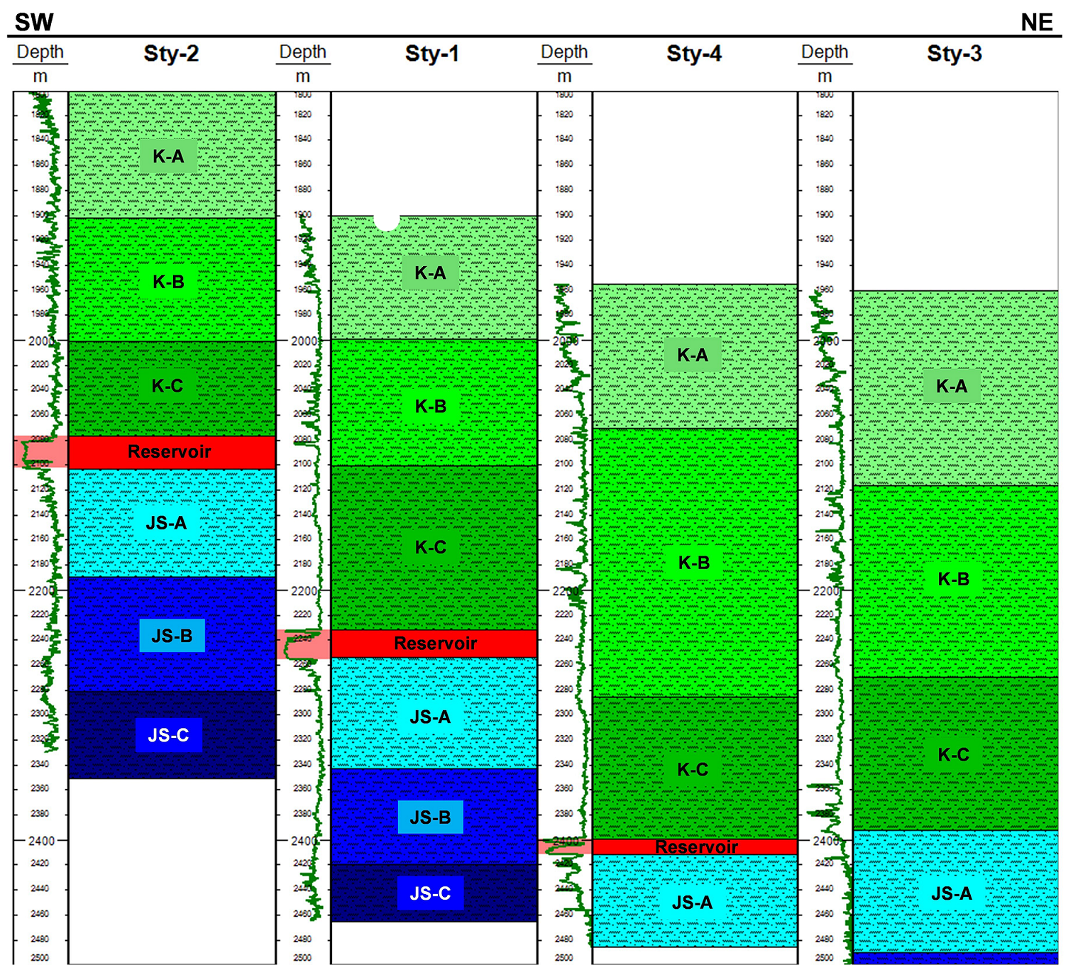
To deploy a field application of the proposed methodology, we used available stacked seismic information of the Stybarrow deepwater field, as well as the information of four wells (Stybarrow-1, Stybarrow-2, Stybarrow-3, and Stybarrow-4), from which the geological formations overlying and underlying the Lower Cretaceous reservoir were selected. The measured depths of wells range from the sea level to 2,100 m and 2,400 m approximately (Figure 2).
1.2.1. Lithology units
A selection of homologated stratigraphic peaks determined from qualitative analysis of the gamma-ray log was made for the four wells used in the proposed methodology (Figure 2). It derived from the little homogeneity in the information available. The available well logs of the Stybarrow-1, Stybarrow-2, Stybarrow-3, and Stybarrow-4 wells in the study area with which the proposed methodology are shown in Table 1.
Table 1 Geophysical logs were available for the wells in the study area. These logs are essential to construct a petroelastic model.
| Well Log | Sty-1 | Sty-2 | Sty-3 | Sty-4 |
|---|---|---|---|---|
| Interval [m] | 1,906-2,460 | 1,800-2,350 | 1,960-2,500 | 1,955-2,485 |
| GR | ♦ | ♦ | ♦ | ♦ |
| RHOB | ♦ | ♦ | ♦ | ♦ |
| Vp | ♦ | ♦ | ♦ | ♦ |
| Vs | ♦ | ♦ |
In Figure 2, the GR log of the four wells in the Stybarrow field is displayed according to their geographic position from SW to NE, Stybarrow-2 (Sty-2), Stybarrow-1 (Sty-1), Stybarrow-4 (Sty-4), and Stybarrow-3 (Sty-3). Also, the reservoir zones penetrated by each well were highlighted with orange shading, highlighting that the Sty-3 no longer cut the reservoir, becoming a delimiting well of the field. As the Sty-1 well has complete information, it was from the results obtained for this well that the results for the other wells and seismic data of the area were calibrated.
1.2.2. Well and seismic inversion data
Herein, we used well data and volumes of inverted elastic parameters provided by Stanford University. The detailed process of seismic inversion modeling is described in Arévalo-López (2017). The inversion process by which the volumes of Ip, Is, and RHOB were obtained is called simultaneous impedance inversion, performed using a constrained sparse-spike inversion algorithm based on the optimization of the L1 norm. This algorithm creates an ensemble of elastic models using multiple partial angle stacks of seismic data (Areválo-López and Dvorkin, 2017).
A set of elastic models using multiple seismic partial angle stacks were generated in Arevalo-López (2017). To achieve this, Aki-Richards equations were used to compute the reflection coefficients at seismic scale, while at well scale (low frequency), P and S velocities are used for the elastic model. Inversion process usually includes QC on input data, cross correlation between the angle stacks for obtaining time-aligned stacks, seismic-to-well tie, wavelet extraction for each angle gathers, horizon interpretation based on the near-stack amplitude, well- and horizon-based low frequency models of Ip, Is, and density of the earth model, inversion parameter optimization, and quality control of the inversion results.
Inversion parameters were optimized to obtain the best fit between the seismically derived values and the data from Well Sty-1. Subsequently, these parameters were used to obtain the simultaneous impedance inversion for the entire seismic cube. The most critical optimization parameter was the "contrast mismatch" that controls the variance of the elastic parameters between the inversion results and the low-frequency well data (Figure 3).
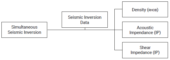
Figure 3 The sequence used to obtain volumes of elastic properties through simultaneous Seismic Inversion (Arévalo-López, 2017).
According to Arévalo-López (2017), the key to obtaining an acceptable seismic inversion is to match the seismically derived Poisson's ratio with the same parameter calculated from well-log data.
2. Petroelastic and Brittleness workflows
2.1. Petroelastic model
This study extended the 1D methodology to implement self-consistent models SCM proposed by Nicolás-López and Valdiviezo-Mijangos (2016) to a 3D petroelastic workflow for lithotype interpretation. SCM was applied to obtain rock's elastic effective properties considering a heterogeneous medium of inclusions (minerals, fluids, or organic matter) for different porosity scenarios. The self-consistent method equations introduced by Sabina and Willis (1988) are non-linear; Valdiviezo-Mijangos and Nicolás-López (2014) solved them with the fixed-point method. When obtaining the solution of the equations, it is assumed that the properties of the rock μ, κ and ρ of a homogeneous system become properties of a heterogeneous system, which are called effective properties
Self-consistent equations for n inclusions are,
where
The self-consistent equations, (1) to (3), were used to construct the rock physics templates RPT in terms of Mu-Rho
2.2. Brittleness models
This work proposed the integrated analysis of lithology's petroelastic interpretation and brittleness evaluation. Elastic parameters
Brittleness index based on Young's modulus (BIE)
This brittleness index is defined by normalization of Young's modulus, taking as its limits the maximum and minimum values of a sedimentary column. In an (E - v) cross-plot, the results usually generate horizontal straight lines because E only varies. BIE is calculated with the following equation,
where E is Young's modulus, Emin is the minimum Young's modulus, and Emax is the maximum Young's modulus. For practical applications, higher values of Young's modulus are related to brittle formations and lower to ductile formations.
Brittleness index based on Poisson's ratio (BIv)
The normalization considers Poisson's ratio from a sedimentary column's maximum and minimum values. Poisson's ratio always has values between 0 and 0.5. This parameter generates vertical straight lines when superimposed on (E - v) cross-plot. It is computed with the following equation,
where v is Poisson's ratio, vmin is the minimum Poisson's ratio, and vmax is the maximum Poisson's ratio. Higher values of Poisson's ratio are always linked to ductile formations and lower to brittle formations.
Average Brittleness index (BA)
As for heuristics, BIE and BIv must be considered to improve brittleness evaluation. Therefore, BA is determined via the linear average between the values of BIE and BIv. This parameter generates oblique straight lines when they are superimposed on (E - v) cross-plot and with which can be performed brittleness analysis. The average brittleness index is obtained with the following expression,
where BIE and BIv were defined in equations (6) and (7).
2.3. Workflow for 1D-3D lithotype interpretation
The proposed workflow for 1D-3D lithotype interpretation is based on rock physics templates RPT which have risen as efficient tools for lithotype interpretation (Nicolas-López et al., 2019). They were constructed similarly described in Nicolás-López and Valdiviezo-Mijangos (2016). Therefore, a new workflow for 3D lithotype interpretation was set up. The lithologies were identified from their 1D-3D elastic properties computed at well and field scale. It is worth mentioning that the same calibrated
In Figure 4, the steps for 1D-3D lithotype interpretation are shown. First, the geometry and consistency of data clouds of petroelastic parameters and density were validated for well and field scales. Next, supervised quality control must be conducted for seismic inversion data and well logs. Finally, the missed data were correlated, honoring the lithology reported in analog wells. Next,
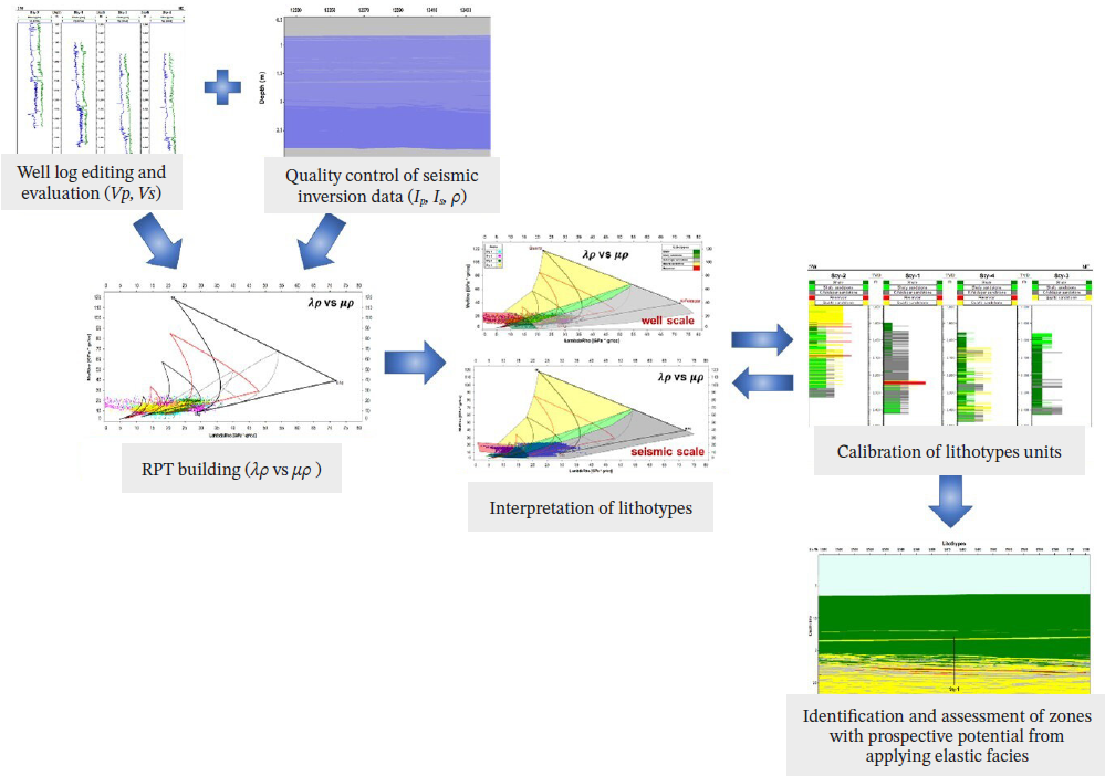
Figure 4 Workflow for 1D-3D lithotype interpretation using ternary rock physics templates. Petroelastic analysis sequence to relate seismic with well logs for obtaining lithotype logs and volume of lithotypes. Ternary rock physics templates were generated considering the 1D methodology described in Nicolás-López and Valdiviezo-Mijangos (2016).
2.4. Workflow for 1D-3D brittleness analysis
For well and field scale, lithology interpretation was suggested by calibrated
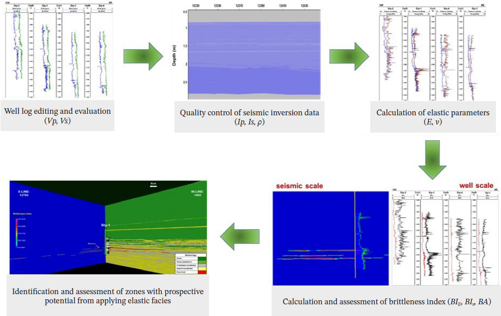
Figure 5 Novel workflow for 1D-3D brittleness analysis for identifying areas with reservoir potential using enhanced 1D brittleness methodology (Lizcano et al., 2018).
3. Results
3.1. Characterization of density and rock's elastic properties
1D-3D petroelastic interpretation and brittleness workflows require a rigorous characterization of density and rock's elastic properties. The required curves to determine elastic properties that will be scaled to seismic information were mainly wet bulk density RHOB, compressional Vp, and shear Vs wave velocities. In this case study, they were available for the Sty-1 and Sty-3 wells (Figure 6). In Sty-2 and Sty-4 wells, it is solely accounted with RHOB and Vp.
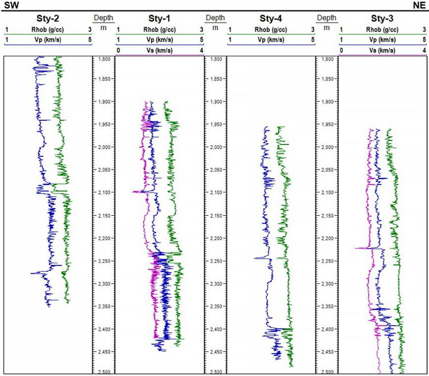
Figure 6 Logs of density and elastic parameters, Vp nd Vs are shown. Wave velocities were calculated from transit time logs. Shear wave velocity Vs was solely available in Sty-1 and Sty-3.
Therefore, it was necessary to compute Vs data for all wells involved in the novel petroelastic modeling proposed. To obtain Vs values with an acceptable accuracy to Sty-2 and Sty-4 wells, a neural networks NN methodology like the one proposed by López-Aguirre et al. (2020) was followed. Herein, Vs curves of Sty-1 and Sty-3 wells with a vertical resolution of 0.1524 m were used as data in training mode; while the wells that did not have Vs were included with a lower vertical resolution (2 m) in the data set defined like test mode. After the NN process was executed, Vs curves for Sty-1 and Sty-3 were modeled (Figure 7). Then, the analysis results for the training wells were compared with the hard data with which a high correlation was obtained. Finally, Vs curves were obtained for the wells that did not have them.
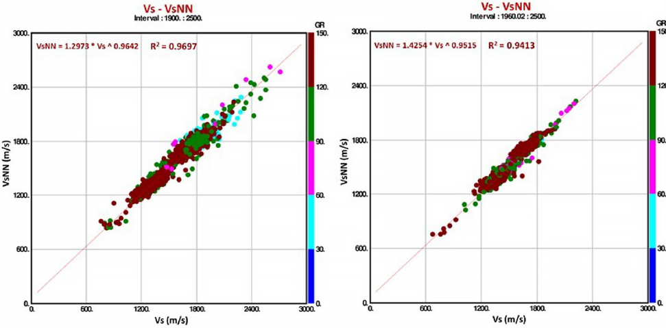
Figure 7 Analysis of the Vs results obtained from neural networks NN. The left figure shows Vs results obtained for the Sty-1, while the right figure shows the results of Vs for the Sty-3 well.
Figure 8 shows the validation of Vs results obtained with NN against actual Vs logs for the Sty-1 and Sty-3 wells. The relationships obtained are those mentioned in the following equations,
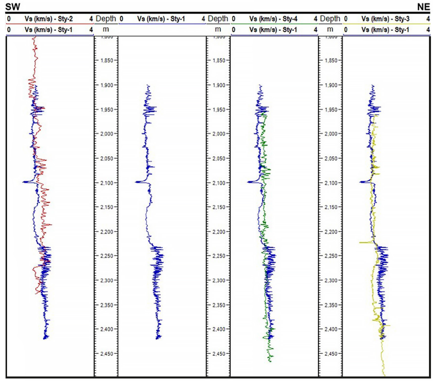
Figure 8 Value-range-based calibration of modeled Vs well logs. Sty-1 is the correlation well for qualitative analysis in tracks.
Next, Vs logs calculated with NN for Sty-2 and Sty-4 wells also have equivalent accuracy of around 95%. In addition, the value range of the four Vs curves estimated with NN is qualitatively placed in context using Sty-1 Vs log, Figure 8. After these realizations of Vs, we have completed the set of density RHOB, compressional Vp, and shear Vs wave velocity for petroelastic interpretation of lithology columns.
3.2. Petroelastic parameters
The elastic parameters Mu-Rho
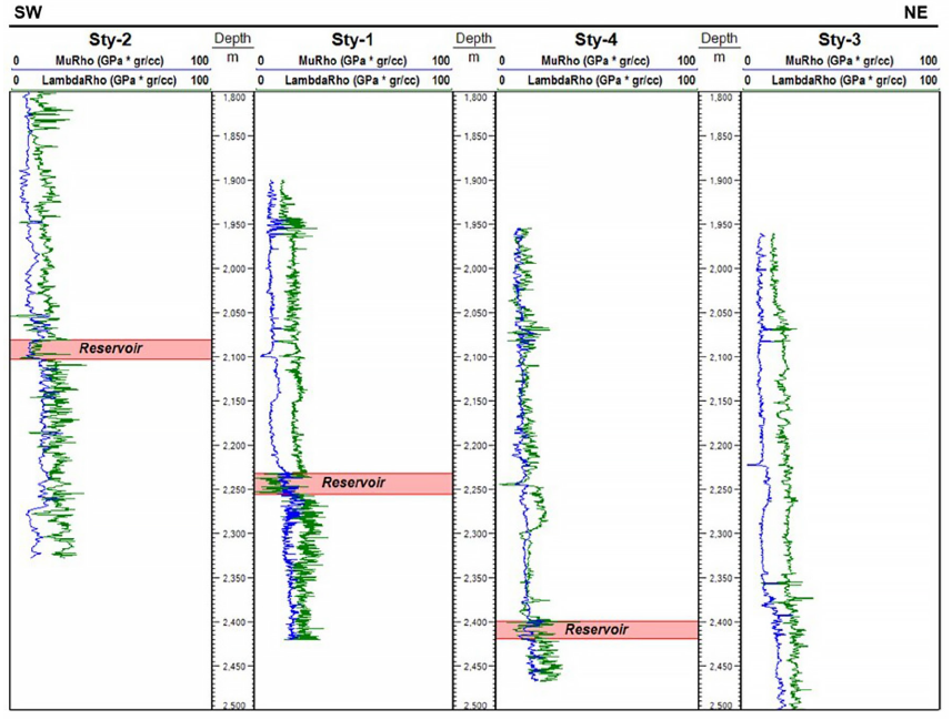
Figure 9 The elastic parameters, Mu-Rho
3.3. 1D petroelastic model for lithotype interpretation
RPT-based interpretation of lithotypes usually starts with defining lithology classification from the field description reported (Nicolás et al., 2019). From the geological information of the study area, the lithologies are linked to dominant minerals, i.e., shale is related to clay minerals, and sandstone to quartz. Sandstones can also be discriminated via the content of the second dominant mineral, Table 2. Therefore, the column was primarily defined by lithologies considering mineralogy content.
Table 2 Lithotypes related to rock's mineral composition. The classification used for 1D-3D lithotype interpretation on well logs and seismic inversion volumes. Feld: Feldspar, K: Potassium, and Qz: Quartz.
| Lithology | Description |
|---|---|
| Shale | Clays > 50% > Quartz, K-Feldspar |
| Shaly Sandstone | Quartz, K-Feldspar ≤ 50% ≤ Clays |
| Feld K Sandstone | Quartz, Clays ≤ 50% ≤ K-Feldspar |
| Qz-Sandstone | Quartz > 50% > K-Feldspar, Clays |
After defining the lithologies that constitute the lithology column, the elastic properties of three dominant minerals were determined to build the specific RPT for the study area. First, we defined two siliciclastic minerals (quartz and potassium feldspar) and one argillaceous mineral (clay), taking information on the three types of clay reported in the case study. Next, a weighted average was calculated for illite/smectite, kaolinite, and chlorite to define clay's elastic properties. Finally, reference values were set for the dominant minerals: quartz, potassium feldspars, and clay, as shown in Table 3.
Table 3 Elastic properties of clays and the dominant rock minerals to build the specific ternary RPT for 1D-3D lithology interpretation.
For the construction of RPT in terms of
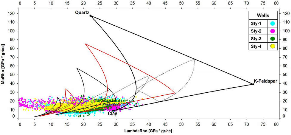
Figure 10 Construction of
In Figure 10, the elastic responses of wells from Figure 9 are plotted together with RPT. The point cloud of each color used corresponds to the elastic information of each of the four wells in the study area. Thus, the blue points correspond to Sty-1, green points to Sty-2, red points to Sty-3 well, and yellow points to Sty-4 well. The
Once the characterization of the ternary RPT with elastic information of the four wells was achieved, Figure 11, the petroelastic interpretation of lithotypes was carried out. At this point, lithologies are defined by elastic responses of rock mixtures where the elastic contribution of pure minerals is considered. In Figure 11, the superimposed zones are mainly guided by the vertices of ternary plots. These are related to lithotypes described in Table 2 as follows: the yellow zone is trending to quartz vertex; therefore, quartz sandstone is straightforwardly discretized; the red zone is for the reservoir and is linked to sandstones, high porosities, and pore-filling fluid; green zone for shales is biased by clay vertex, grey zone is for k-feldspar sandstone, and the light green zone is for shaly sandstone.
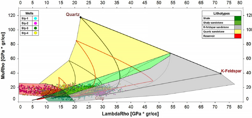
Figure 11 Ternary RPT shows the resulting lithotypes for the 1D model for the four wells, which would later be scaled to seismic to obtain a 3D geological model.
Zones portrayed in Figure 11 are used to select points and differentiate between themselves. The filtered points are separately related to each lithotype for 1D petroelastic lithology interpretation. A third fundamental property, apart from
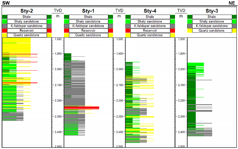
Figure 12 1D petroelastic interpretation of lithologie columns. Cross-section correlation of lithology units colored with zones of Figure 11.
3.4. 3D petroelastic model for lithotype volume construction
1D petroelastic interpretation of lithologies is the main foundation for 3D petroelastic interpretation because the data design and visualization are analogous. In Figure 13, the validated ternary RPT was used in the same fashion as Figure 11. However, at this stage, the input data were calibrated volumes in terms of
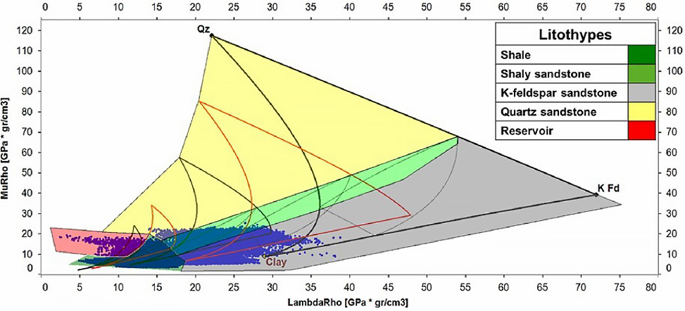
Figure 13 Shows the resulting lithotypes for the 1D model for the four wells, which would later be scaled to seismic to obtain a 3D geological model.
The shaded zones were used to select and characterize volumes of seismic inversion data in
In Figure 15, stratal slice analysis focused on the spatial distribution of the reservoir was performed. Remember that this is a 3D visualization of the selection of intervals in red from Figure 13. These points are colored zones in red in Figures 14 and 15. Sty-1 well clearly dropped in the best zone of the reservoir because it landed in the broader area in red. Commercial output is often linked to the vast presence of pore-filling fluid. In contrast, Sty-2 and Sty-3 were drilled in a sparse area in red. Sty-4, a re-entry of Sty-3, also dropped in a scarce area in red. The proposed 1D-3D interpretation of lithologies integrated with field and production well reports can assist in defining hydrocarbon-rich zones within the target stratum.
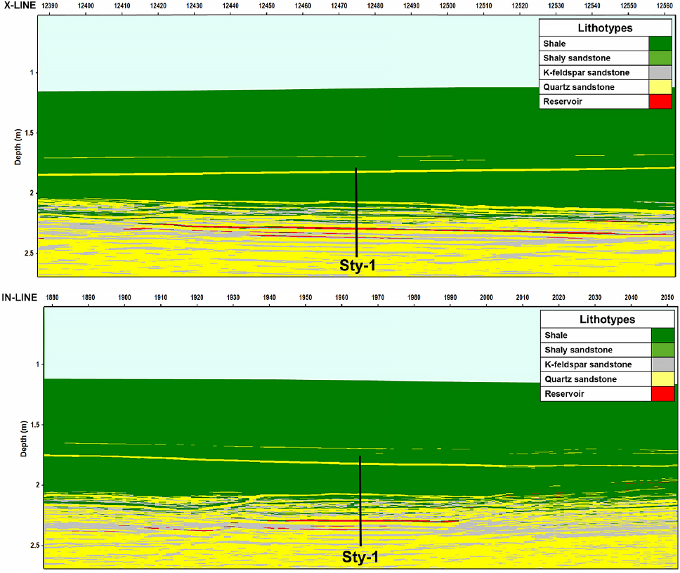
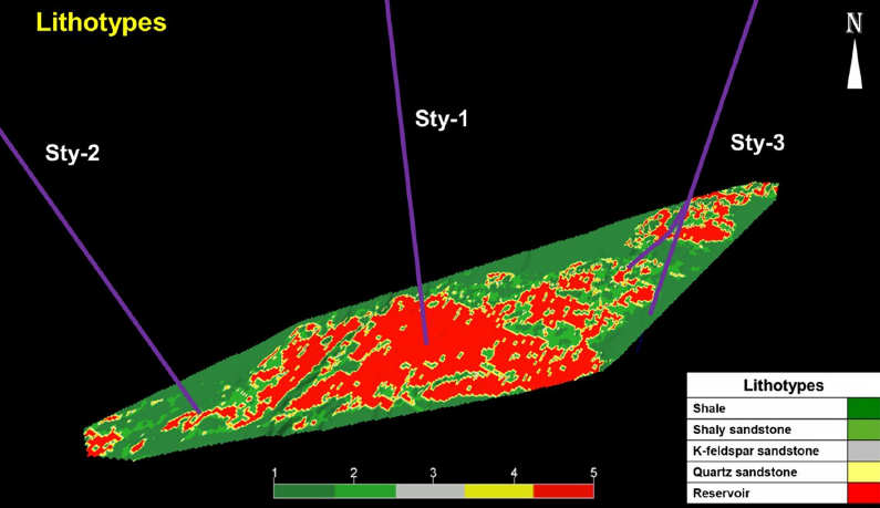
Figure 15 Stratal slice of reservoir identified by the rock physics templates RPT. The zone in red in Figure 13 encompasses the points distributed within the stratal slice.
3.5. 1D brittleness model
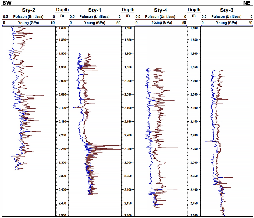
Integrating the petroelastic model of lithotypes and brittleness modeling is the major novelty of this research. Brittleness modeling reinforces 1D-3D petroelastic interpretation by quantifying brittleness in hydrocarbon-rich zones. Brittleness evaluation carried out based on Young's modulus E and Poisson's ratio v is well accepted in the oil industry, Section 2.2. Lab tests, well logs, and seismic inversion volumes can obtain these elastic parameters. Herein, the first step is to define the maximum and minimum values of E and v. In Table 5, the corresponding values are shown. They are related to dominant minerals with the highest and lowest values for E and v.
Next, E and v curves were calculated using geophysical logs modeled in section 3.1. The elastic parameters obtained for the wells are those presented in Figure 16.
With the elastic parameters defined and calculated for each well, E and v curves are normalized by applying equations 6 and 7. Brittleness indexes based on Young's modulus BIE and Poisson's ratios BIV are portrayed in Figure 17. They are qualitative indicators because they depend on the maximum and minimum values used. For instance, we used limits referenced in Table 4; however, the curve behavior will not change when other limits are used. The critical point is honoring the elastic properties of the most brittle and ductile formations.
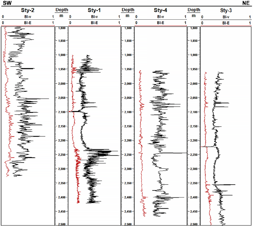
Table 4 Maximum and minimum values to E and v for brittleness analysis of the wells of the study case.
| Parameter | Max | Min |
|---|---|---|
| E (GPa) | 95.4 | 2.8 |
| v (Unitless) | 0.44 | 0.07 |
Note that normalized profiles of BIE are lesser than BIV in wells evaluated. This issue is because, in the discretization, the theoretical value of quartz with porosity equal to 0 was used as the maximum value for E. Therefore, we suggest using core data when available to maximum and minimum values for E and v at target formation. Finally, computing the arithmetic average of BIE and BIV with equation (8), the BA brittleness index was obtained and used to discriminate intervals with greater and lesser brittleness. Reservoir intervals reported are references to the brittleness quantification considering the elastic contribution of pore-filling fluid, Figure 18. Sty-1 reported a potent reservoir interval in contrast to Sty-3, which landed out of the hydrocarbon-rich zone. These well behaviors were linked to the performance of BA curves. Based on a qualitative interpretation of BA and the oil field data, the higher values
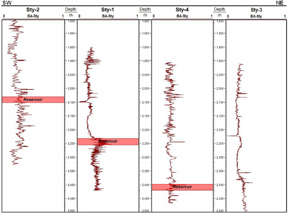
Figure 18 Brittleness average (BA) based on a simple average of BIE and BIv to wells in the case study. Reservoir depths were used to calibrate the ranges of BA qualitatively.
It was obtained, and in the case of the Sty-1 well, the identification of the hydrocarbon zone. In Figure 18, the results of BA are shown.
3.6. 3D brittleness model
In the same fashion that was scaled 1D to 3D petroelastic interpretation of lithotypes, sections 3.3 and 3.4., 1D brittleness modeling was scaled to 3D brittleness modeling. Herein, 3D brittleness analysis was executed using volumes of Young's modulus and Poisson's ratio. These volumes came from seismic inversion tied with the area wells (Arévalo-López, 2017). Drawbacks about using data at different scales were solved in that step. For brevity, figures of intermediate normalizations of BIE and BIv were skipped. Results of 3D brittleness analysis based on BA are shown at the target stratum. Reservoir zones linked to BA were also investigated as an indicator of saturated zones. The latter represents an outstanding feature of lithotypes and brittleness workflows proposed.
Figure 19 shows 1D-3D brittleness modeling conducted on in-line and x-line corresponding to the intersection with the Sty-1. Zones in red denote higher values of the BA brittleness index, consistent with the 1D brittleness analysis performed on Sty-1. The horizontal spatial distribution is related to the lateral continuity of brittle intervals at the target stratum, and vertical variations can underpin well paths to drill the most significant number of brittle intervals.
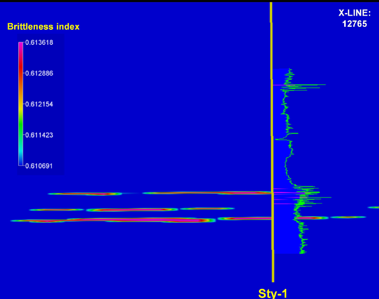
Figure 19 Brittle zones in red from 1D-3D brittleness analysis of the case study. Sty-1 is used as a correlation well.
The same stratal slice, Figure 15, is used to portray the spatial distribution of brittle zones and landing area of the well paths, Figure 20. Regions in red were discriminated by cutting the higher values of the BA brittleness index. For example, at the target stratum, Sty-1 was placed into a sizeable brittle zone; Sty-2 and Sty-3 were drilled in poor brittleness zones; and Sty-4, a re-entry well from Sty-3, was redirected to an area with higher brittleness. This brittleness analysis carried out on wells and stratal slices, features the BA brittleness index as a new reservoir indicator.
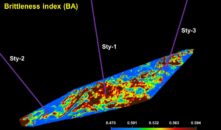
Figure 20 Reservoir identification using the brittleness index modeling. BA index was set out as a reservoir indicator in terrigenous formations.
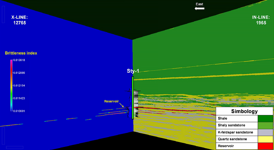
Finally, in Figure 21, the integration of workflow results of both petroelastic interpretation and brittleness analysis are shown. The in-line: 1965 and cross-line: 12765 corresponds to Sty-1, and the reservoir zone in red was identified at well scale and delineated at seismic scale. 3D visualization of lithotype distribution, Figure 15, and higher values of
4. Discussion
Following the proposed methodology (Section 2, Figure 4), it was possible to determine, with the support of the
5. Conclusions
The results obtained from the lithotypes, at the well level and the seismic level, permit the identification of the reservoir zones, which were concordant at both levels of analysis. The effectiveness of the petroelastic workflow proposed as a complement to calibrate conventional exploratory analyzes was ascertained. The proposed methodology supported in the RPTs established the identification of lithologies at the log level, consistent with published results, which assisted defining and scaling the lithologies to the seismic one, with volumes of valuable subsurface information obtained.
Applying the proposed methodology, it was possible to determine the spatial distribution of the reservoir, which honors the results obtained independently for each of the wells, as well as confirm what has been reported in the literature for the study area. In the same way, the methodology allowed identifying the zones in which, according to what was reported, there are no reservoir conditions, as is the case of the Sty-3 well. It has also been possible to contribute to the quantitative seismic interpretation from the results obtained from the brittleness modeling both at the well and seismic levels. With the above, it is noted that this method has great potential since it is through calculations and not the interpreter's subjectivity that the zones of the potential reservoir were differentiated.
In the lithological interpretation carried out with the RPT, the areas with hydrocarbon content that allowed their identification were attenuated. Additionally, the workflow for brittleness analysis was applied at the well and seismic level, which confirmed the areas of the reservoir with the best conditions for the prospective location of wells. While in the quantitative estimation carried out with the brittleness modeling, it was determined that the reservoir zones are found in BA brittleness index greater than 0.5. Also, in the application of the said methodology, it is the BIv brittleness obtained for Poisson's ratio, which is the most sensitive to attenuation due to hydrocarbon content, for which it is proposed to carry out tests in which BA is obtained, through averages of a different nature than arithmetic to refine the areas of potential reservoir more.

