


 (pdf)
(pdf)


 SciELO
  SciELO
 Permalink
1. Introduction
Drought is defined as a reduction in precipitation compared to the annual average and is caused by prolonged periods of below-normal rainfall. It can affect various aspects of the water cycle and as a consequence, one type of drought can become another over time, being a phenomenon that operates at different scales and is influenced by the speed with which a specific area responds to changes. Therefore, the time scale plays a critical role in determining the specific type of drought that is occurring. The different time scales help classify droughts into meteorological (1 month), agricultural (3-6 months), and hydrological (12-24 months) categories. Specifically, hydrological drought occurs when the levels of surface reservoirs such as rivers and lakes gradually decrease, sometimes even depleting completely (Esparza, 2014). Classifying droughts based on these time scales is essential to accurately assess the severity and type of drought in a given region. Drought is also a phenomenon that occurs in cycles in all climates worldwide, although with varying intensity and frequency. In Mexico, droughts occur on average once every 20 years, leading to a hydrological imbalance in the water cycle due to insufficient resource availability.
The lack of rainfall in different regions of the state of Chihuahua has resulted in drought occurring in 64 out of the 67 municipalities of the territory, as described by the Drought Monitor in Mexico in its report published on July 4, 2022. The report details that the state is experiencing all five classifications of drought. The three watersheds that supply water to the municipalities in the region were affected by severe, extreme, or exceptional drought conditions, with the city of Chihuahua experiencing extreme drought (SMN, 2022).
One of the most alarming consequences of drought is the damage to agriculture in recent years. The direct impact of these losses is reflected in the rising prices of basic commodities. Crop loss, in turn, increases the risk of widespread famine due to the inability to ensure a stable food supply. Furthermore, the situation has generated tensions and conflicts at various levels and locations.
The Standardized Precipitation Evapotranspiration Index (SPEI) aims to measure the level of drought at a specific location. It is based on precipitation and temperature data and combines multiscale character with the ability to incorporate temperature variability. Machine learning efficiently captures knowledge within the data to make decisions based on it.
In the work of Belayneh and Adamowski (2013), machine learning techniques for Artificial Neural Networks (ANN), Support Vector Regression (SVR), and Wavelet Analysis (WA) were investigated in the Awash River basin in Ethiopia using the Standardized Precipitation Index (SPI). The results show that the WA-ANN is the most accurate model for predicting the values of SPI-3 and SPI-6, with coefficient of determination (R2) values greater than 0.96 and root mean squared error (RMSE) less than 0.025. The study of Zhang et al. (2019) took place in Shaanxi, China. The Distributed Lag Non-Linear Models (DLNM), ANN model, and Extreme Gradient Boosting (XGBoost) model were constructed, and their validations were compared to predict SPEI one to six months in advance. As a result, the XGBoost model was superior, with R2 values between 0.68-0.82, 0.72-0.89, 0.81-0.92, and 0.84-0.95 in three, six, nine, and 12 months, respectively. The study of Mokhtar et al. (2021) took place on the Tibetan Plateau, China considering SPEI-3 and SPEI-6 to develop the random forest (RF) algorithm, XGBoost, convolutional neural networks (CNN), and Long-Short Term Memory (LSTM) models.
Seven scenarios of various combinations of climate variables were adopted as input to build the models. The best model was the SPEI-3 XGBoost, which obtained an MBE of 0.04 and a Nash-Sutcliffe efficiency (NSE) of 0.70. The study of Dikshit et al. (2021) uses LSTM networks to predict SPEI-1 and SPEI-3. The model was compared to the RF algorithm and applied in Australia’s New South Wales region. The model achieved an R2 value of more than 0.99 for the SPEI-1 and SPEI-3. In the work of Hernández (2021), ANNs were evaluated in the Sonora River basin, Mexico, using SPI and SPEI at time scales of three, six, 12, and 24 months. The results showed an average R2 of 0.76, and it was observed that the performance of SPEI was better than that of SPI and increased with increasing time scale.
The existing works on machine learning algorithms to predict drought are not exactly focused on hydrological drought, meaning they do not focus on obtaining the best results on the 12- and 24-month time scales. As the SPEI is the improved version of the SPI, this work specializes in the SPEI to obtain more precise and updated information, unlike other studies. The few works in which SPEI and machine learning algorithms work together train only one type of algorithm. Therefore, the results have limitations. Given this, the study’s objective is to anticipate extreme situations by analyzing drought cycles within the city of Chihuahua using a database of the monthly SPEI 12 and SPEI 24 indices from 1901 to 2020. This analysis employs the machine learning methods of SVR, ANN, and LSTM to predict droughts, mitigate their impact, and visualize future trends.
2. Materials and method
2.1 Standardized Precipitation Evapotranspiration Index (SPEI)
The purpose of the SPEI is to measure the level of drought at a specific location. Its multiscale nature makes it useful for various scientific disciplines because it can measure severity based on its intensity and duration and identify the onset and end of drought episodes. It can be calculated across a wide range of climates, and a crucial advantage over other indices is that its multiscale characteristics allow it to identify different types of droughts and impacts in the context of global warming (Vicente-Serrano et al., 2010). The specific definition and classification of drought based on SPEI are shown in Table I.
Table I Categorization of SPEI values.
| Category | SPEI |
| Extremely wet | Greater than 2.0 |
| Very wet | De 1.50 a 1.99 |
| Moderately wet | De 1.00 a 1.49 |
| Near normal | De -0.99 a 0.99 |
| Moderately dry | De -1.00 a -1.49 |
| Very dry | De -1.50 a -1.99 |
| Extremely dry | Less than -2.0 |
SPEI: Standardized Precipitation Evapotranspiration Index.
2.1.1 Calculating the SPEI
The probability density function of a three-parameter log-logistic distributed variable is expressed as follows:
where α, β, and γ are scale, shape, and location parameters, respectively, for values of D within the range γ > D < ∞.
The parameters of the log-logistic distribution can be obtained by following the method (Singh et al., 1993):
where Γ(β) is the gamma function of β.
The probability distribution function of D according to the log-logistic distribution is given by:
With F(x), the SPEI can be easily obtained as the standardized F(x) values. For example, following the classical approximation of Abramowitz and Stegun (1964):
where
For P ≤ 0.5, where P is the probability of exceeding a certain value D, P = 1 - F(x). If P > 0.5, it is replaced by 1 - P, and the sign of the resulting SPEI is inverted. The constants are:
C 0 = 2.515517, C 1 = 0.802853, C 2 = 0.010328, d 1 = 1.432788, d 2 = 0.189269, and d 3 = 0.001308.
2.2 Machine learning algorithms
In the second half of the 20th century, machine learning evolved as a subfield of artificial intelligence, offering a more efficient alternative for capturing knowledge from data. Instead of relying on humans to manually derive rules and construct models through the analysis of vast datasets, machine learning identifies patterns of statistical repetitions to gradually improve the performance of predictive models and make data-driven decisions.
2.2.1 Artificial Neural Networks (ANN)
It is well known that learning takes place within the brain. To understand this process, it is necessary to comprehend the basic element, the neuron. Neurons perform chemical transmissions within the brain, carrying information that can either increase or decrease the neuron’s electrical potential. If this membrane potential reaches a certain threshold, the neuron fires a pulse of specific strength and duration sent down the axon. The axon, in turn, branches out into various connections to other neurons, linking to each of them through synapses.
McCulloch and Pitts (1943) introduced the first mathematical model of an artificial neuron that could capture the essential elements of how a neuron functions by emulating its operations and determining whether it should fire. Subsequently, Frank Rosenblatt (1958) invented the first neural network known as the Perceptron, and later, Bernard Widrow and Ted Hoff (1997) published the adaptive linear neuron algorithm (ADALINE) algorithm, which can be considered an improvement. This algorithm consisted of a collection of McCulloch-Pitt neurons and inputs and weights.
ADALINE is particularly interesting because it illustrates the concept of defining and minimizing cost functions, laying the foundation for understanding more advanced machine learning algorithms for classification and regression models. In addition, backpropagation is the process that seeks the best parameters to reduce the network’s error.
2.2.2 Long Short-Term Memory (LSTM)
Juergen Schmidhuber (1997) introduced the so-called LSTM units, which are managed in memory blocks with self-connections. Their advantage lies in their ability to store the temporal state of the network. LSTM cells have special multiplicative units called gates, which control the data flow. The components of memory blocks include the input gate (it), which controls the flow of input activations into a cell; the output gate (ot), where the flow of output from the cell’s activation is controlled; and the forget gate (ft), where the input information is filtered (xt) and the previous output is filtered (Fig. 1).
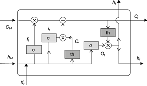
Fig. 1 Graphic representation of the structure of a Long-Short Term Memory (LSTM) model where: x n is the input of the model, h n is the output, f t is the forget gate, i t is the input gate y ĉ t is the update cell, c t is the state cell and o t is the output gate. Obtained from Zhu et al. (2020).
2.2.3 Support Vector Regression (SVR)
SVR uses the perceptron algorithm to minimize classification errors. Its objective is to maximize the distance between the separation hyperplane and the closest training samples to it, referred to as support vectors. In a dataset where it is not possible to separate the samples using a linear hyperplane as a boundary with the assistance of linear models, kernel methods attempt to create nonlinear combinations of features to project them into a higher-dimensional space through mapping, where linear separation becomes feasible (Fig. 2).
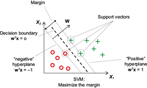
Fig. 2 Graphic representation of the support vector machine’s (SVM) work and the intention to maximize the margin. Obtained from Raschka (2015).
2.3 Obtaining climatological data
The dataset containing monthly SPEI 12 and SPEI 24 data will be collected through the Global SPEI Database project (https://spei.csic.es/) from the Climatology and Services Laboratory. This involves searching for geographical coordinates on the official website, selecting the data type sought, and downloading the information in .csv format. The type of data is shown in Table II.
Table II SPEI 12 and SPEI 24 input data.
| Date | SPEI 12 | SPEI 24 |
| 1901-01-16 | -0.25413 | 0.94915 |
| 1901-02-15 | -0.09160 | 0.92983 |
| 1901-03-16 | -0.36882 | 0.92330 |
| 1901-04-16 | -0.42440 | 0.91418 |
| - | - | - |
| 2020-09-16 | -1.56340 | -1.60910 |
| 2020-10-16 | -1.94560 | -1.86140 |
| 2020-11-16 | -2.18390 | -1.92440 |
| 2020-12-16 | -2.24050 | -1.96930 |
SPEI: Standardized Precipitation Evapotranspiration Index.
2.4 Preprocessing
Once the file is obtained, it is scaled so that the data is no longer between -3 and 3, but the minimum data value becomes 0, and the maximum becomes 1 (a process known as normalization). This reduces the computational cost associated with working with a variety of values.
Due to the nature of the data, this analysis is categorized as a time series. The way to work with such projects involves creating small windows of data, which in the case being discussed consists of 12 months because a cycle repeats yearly. These windows are formed with data from t = 0 to t = 11, and the last column is considered the one to be predicted or, in other words, the label. This is how all the windows are created from the database, overlapping. The previous windows help serve as feature vectors along with the label. This is how subseries are generated.
2.5 Data import
A series of experiments were conducted to find the best configurations for the three proposed methods and the two types of SPEI. From the results, the top two architectures for each method were selected and analyzed in the obtained results.
2.5.1 ANN
The dataset was split into 90% for training and 10% for testing. The Adamax optimizer was used. The networks were trained for 20 epochs with a batch size of 1. The values of ‘n’ were based on the configurations that yielded the best results in the consulted articles, resulting in a total of 100 different cases (Table III).
2.5.2 LSTM
Same configuration as in ANN, resulting in a total of 250 different cases (Table IV).
Table IV Structure of Long-Short Term Memory (LSTM) models.
| Input | LSTM | Hidden 1 | Dropout | Hidden 2 | Output |
| 12 | 1 | 1, 2, 4, 8, 16 | 0.5 | 1, 2, 4, 8, 16 | 1 |
| 12 | 2 | 1, 2, 4, 8, 16 | 0.5 | 1, 2, 4, 8, 16 | 1 |
| 12 | 4 | 1, 2, 4, 8, 16 | 0.5 | 1, 2, 4, 8, 16 | 1 |
| 12 | 8 | 1, 2, 4, 8, 16 | 0.5 | 1, 2, 4, 8, 16 | 1 |
| 12 | 16 | 1, 2, 4, 8, 16 | 0.5 | 1, 2, 4, 8, 16 | 1 |
| 12 | 32 | 32, 64, 128, 256, 512 | 0.5 | 32, 64, 128, 256, 512 | 1 |
| 12 | 64 | 32, 64, 128, 256, 512 | 0.5 | 32, 64, 128, 256, 512 | 1 |
| 12 | 128 | 32, 64, 128, 256, 512 | 0.5 | 32, 64, 128, 256, 512 | 1 |
| 12 | 256 | 32, 64, 128, 256, 512 | 0.5 | 32, 64, 128, 256, 512 | 1 |
| 12 | 512 | 32, 64, 128, 256, 512 | 0.5 | 32, 64, 128, 256, 512 | 1 |
2.5.3 SVR
The varied parameters included kernel, regularization parameter ‘C’, kernel coefficient ‘Gamma,’ and polynomial degree. This way, five folds were obtained for 128 candidates, resulting in a total of 640 fits (Table V).
2.6 Performance statistics for model evaluation
The model’s performance was evaluated by comparing statistical parameters between predicted and observed data, using the metrics mean bias error (MBE), MAE, MSE, R2, and Kendall’s correlation coefficient.
2.6.1 Mean bias error (MBE)
It is used to estimate the model’s average bias and determine the steps needed to correct the model’s bias.
where N is the total number of samples, P corresponds to the predicted value, and O to the observed value. An MBE equal or near zero indicates that, on average, the model predictions are free of systematic bias. A positive MBE indicates that the model predictions tend to be systematically higher than the actual values, and similarly, a negative MBE indicates that the model predictions tend to be systematically lower than the actual values.
2.6.2 Mean absolute error (MAE)
It is an evaluation metric used with regression models. It involves taking the mean of the absolute values of individual predictive errors across all instances. Each prediction error is the difference between the actual value and the predicted value,
A MAE value equal to 0 would indicate that the model makes perfect predictions, coinciding with the real values in all cases. The closer to 0, the better the accuracy of the model. A relatively high MAE indicates that the model predictions tend to deviate more from the actual values.
2.6.3 Mean squared error (MSE)
It is a quantitative measure of a model’s performance. It is the average value of the cost function, which is the sum of squared errors that is minimized to fit the regression model. MSE is very useful for comparing different regression models or tuning their parameters through grid search and cross-validation.
Like the previous error, a low MSE indicates better model performance but differs in that when squaring the errors, the MSE gives more weight to larger errors.
2.6.4 Coefficient of determination (R 2 )
It can be understood as a standardized version of MSE for better interpretability of the model’s performance:
where Ō is the mean observed value. R2 has a range from 0 to 1. If R2 converges to 1 it is considered a ‘very good’ relationship. When R2 is between 0.8 and 1, it is labeled ‘good’. In the range of 0.6 and 0.8, it is ‘satisfactory’. If lower than 0.6, it is classified as a weak relationship. When a correlation converges to 0, it is considered ‘inefficient’. Finally, if R2 is less than 0, it is considered invalid.
2.6.5 Kendall’s correlation coefficient
The Kendall correlation coefficient evaluates the order relationship between variables, not the magnitude of the difference between them. Unlike the determination coefficient R2, Kendall’s coefficient takes into account the order used in the time series. Therefore, it proves to be widely useful data dependent on a temporal variable. It is a rank-based correlation coefficient known as non-parametric correlation. Its formula is:
where:
Concordat pair: A pair of observations (x 1 , y 1 ) and (x 2 , y 2 ) that follow:
Discordant pair: A pair of observations (x 1 , y 1 ) and (x 2 , y 2 ) that follow:
Tau equal to or close to 1 indicates a perfect positive correlation between the two ordinal variables, which means that there is an increasing monotonous relationship between the classifications of both variables. Tau equal to or close to -1 indicates a perfect negative correlation, and there is a decreasing relationship. Tau equal to or close to 0 indicates that there is no correlation between the two ordinal variables.
3. Results
The best results are presented in Tables VI and VII. Comparison graphs of actual data with predicted values in the validation set and loss graphs for the ANN and LSTM methods are also shown (Figs. 3 and 4).
Table VI Best SPEI 12 configurations, where Hn represents the hidden layers, L the LSTM layer, K the kernel, G the gamma, C the regularization parameter C, and D the degree.
| Method | Parameters | MSE | MAE | MBE | R2 | Kendall’s coefficient |
| ANN | H1: 15, H2: 15 | 0.0053 | 0.0544 | 0.0207 | 0.8461 | 0.7553 |
| ANN | H1: 12, H2: 17 | 0.0052 | 0.0546 | 0.0196 | 0.8470 | 0.7543 |
| LSTM | L: 32, H1: 64, H2: 64 | 0.0055 | 0.0550 | 0.0250 | 0.8407 | 0.7583 |
| LSTM | L: 64, H1: 32, H2: 64 | 0.0054 | 0.0546 | 0.0257 | 0.8425 | 0.7612 |
| SVR | K: poly, G: scale, C: 1, D: 1 | 0.0047 | 0.0517 | 0.0193 | 0.8618 | 0.7620 |
| SVR | K: linear, G: scale, C: 1, D: 1 | 0.0048 | 0.0523 | 0.0209 | 0.8598 | 0.7642 |
SPEI: Standardized Precipitation Evapotranspiration Index; MSE: mean squared error; MAE: mean absolute error; MBE: mean bias error; ANN: Artificial Neural Networks; LSTM: Long-Short Term Memory; SVR: Support Vector Regression.
Table VII Best SPEI 12 configurations, where Hn represents the hidden layers, L the LSTM layer, K the kernel, G the gamma, C the regularization parameter C, and D the degree.
| Method | Parameters | MSE | MAE | MBE | R2 | Kendall |
| ANN | H1: 12, H2: 19 | 0.0029 | 0.0398 | 0.0219 | 0.9096 | 0.8564 |
| ANN | H1: 13, H2: 20 | 0.0028 | 0.0396 | 0.0216 | 0.9112 | 0.8602 |
| LSTM | L: 32, H1: 32, H2: 32 | 0.0022 | 0.0353 | 0.0135 | 0.9293 | 0.8653 |
| LSTM | L: 64, H1: 64, H2: 128 | 0.0027 | 0.0388 | 0.0242 | 0.9157 | 0.8685 |
| SVR | K: poly, G: scale, C: 1, D: 1 | 0.0021 | 0.0356 | 0.0086 | 0.9335 | 0.8436 |
| SVR | K: linear, G: scale, C: 1, D: 1 | 0.0021 | 0.0363 | 0.0080 | 0.9317 | 0.8409 |
SPEI: Standardized Precipitation Evapotranspiration Index; MSE: mean squared error; MAE: mean absolute error; MBE: mean bias error; ANN: Artificial Neural Networks; LSTM: Long-Short Term Memory; SVR: Support Vector Regression.

Fig. 3 Graph of actual SPEI values (black line) and predicted values (red line) from the Support Vector Regression (SVR) model for SPEI 12. Both with scaled gamma, C = 1, Degree = 1, and polynomial kernel. (SPEI: standardized precipitation evapotranspiration index.)
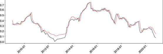
Fig. 4 Graph of real (black line) and predicted (red line) SPEI values from the LSTM model for SPEI 24 with 32-32-32 neurons. (SPEI: Standardized Precipitation Evapotranspiration Index; LSTM: Long-Short Term Memory).
The loss graphs for MSE, obtained epoch by epoch during the training of ANN and LSTM, reveal that the training was stable due to the inverse exponential behavior. This also indicates that the algorithm is learning correctly without overfitting.
3.1 SPEI 12
The ANN algorithms achieved MSE of around 0.005, MAE of 0.054, MBE of 0.020, R2 of 0.84, and Kendall’s coefficient of 0.75. When comparing the two best configurations, it is observed that the 15-15 network outperforms the 12-17 network in the MAE and Kendall’s coefficient categories, while it is inferior in MSE, MBE, and R2. Employing LSTM networks for SPEI 12, MSE of around 0.005, MAE of 0.054, MBE of 0.025, R2 of 0.84, and Kendall’s coefficient of 0.76 were obtained. Comparing the two architectures, the 32-64-64 network surpasses the 64-32-64 network in the MBE category, while it is inferior in all other aspects. Using the SVR method for SPEI 12, MSE of around 0.004, MAE of 0.052, MBE of 0.020, R2 of 0.86, and Kendall’s coefficient of 0.76 were achieved. When comparing the two configurations, the polynomial configuration outperforms the linear one in the MSE, MAE, MBE, and R2 categories while being inferior in Kendall’s coefficient category.
Comparing all the results, for SPEI 12, the polynomial SVR (Fig. 3) dominated all categories except Kendall’s coefficient, where ANN 12-17 performed better. However, there was no significant difference in the values. Unlike the other methods, SVR performed better when facing drastic drops in observed values.
3.2 SPEI 24
Using ANN algorithms, MSE of around 0.002, MAE of 0.039, MBE of 0.021, R2 of 0.91, and Kendall’s coefficient of 0.85 were achieved. In this case, the 13-20 configuration has an advantage in all categories over the 12-19 configuration. Moving on to LSTM networks, MSE of around 0.002, MAE of 0.036, MBE of 0.019, R2 of 0.92, and Kendall’s coefficient of 0.86 were obtained. In this case, the 32-32-32 configuration has an advantage in all categories over the 64-64-128 configuration. When using SVR, MSE of around 0.002, MAE of 0.036, MBE of 0.008, R2 of 0.93, and Kendall’s coefficient of 0.84 were achieved. In this case, the polynomial configuration is better in MAE, R2, and Kendall’s coefficient and inferior in MSE and MBE.
For SPEI 24, the competition is more balanced. The polynomial SVR performed better in MSE and R2, the LSTM 32-32-32 in MAE, the linear SVR in MBE, and the LSTM 64-64-128 in Kendall’s coefficient. In this case, the LSTM 32-32-32 (Fig. 4) is slightly more accurate than the SVR methods.
3.3 Overall interpretation
The observed performances of the models highlight the importance of selecting appropriate architectures for SPEI prediction. Variations in performance metrics offer insights into the model’s abilities to capture complex environmental dynamics. Assessing the robustness of the models over different time intervals reveals the temporal sensitivity of the predictions.
Sensitivity analysis on network architectures and hyperparameters sheds light on the nuanced impact of design choices on model performance. Recognizing the sensitivity of models to these factors is vital to optimize predictive capabilities.
Comparisons between ANN, LSTM, and SVR highlight the nuances of trade-offs associated with each model type. While SVR shows resilience against drastic drops in observed values, ANNs and LSTMs are stronger at capturing specific temporal dependencies.
4. Discussion
In this research, we created predictive models using ANNs, LSTM, and SVR to estimate the temporal scales of SPEI 12 and SPEI 24 from 1901 to 2020 in Chihuahua, Chihuahua, Mexico. A total of 956 experiments were carried out, involving variations in parameters such as the number of neurons, kernel, and polynomial degree, among others. The two best models were chosen for each method, and the outcomes indicated the following performance metrics: MSE = 0.0047, MAE = 0.0517, MBE = 0.0193, R2 = 0.8618, Kendall’s coefficient = 0.7620 for SPEI 12, and MSE = 0.0022, MAE = 0.0353, MBE = 0.0135, R2 = 0.9293, Kendall’s coefficient = 0.8653 for SPEI 24.
As reported by Hernández (2021), it is observed that the precision of the models is better as the time scale increases, probably due to greater short-term variability of the conditions. The improvement in reducing errors from SPEI 12 to SPEI 24 was between 30-50%, and the increase in the other metrics was 7-11%, so the assumption can be complemented. In this study, the performance of the SVR algorithms was very good compared to all the methods used, and as it is unusual to see this technique in other papers, it is interesting to consider that there is an area of opportunity. On the other hand, the XGBoost algorithm has performed outstandingly in several studies and was not tested in this work. Future experiments should consider studying and applying it to improve the accuracy of trained models. Although the purpose of this paper is limited to training machine learning models, the possibility of working on its application opens up.
5. Conclusions
The models developed during the project performed well and were not very different from each other. However, the polynomial SVR achieved greater accuracy in the case of SPEI 12, while LSTM 32-32-32 was slightly better for SPEI 24.
Notably, in all models, there was a challenging peak to adapt to and predict. This value corresponds to the smallest in the database (indicating the highest presence of drought) and is located in January 2011, which was the driest year in recent times in the Mexican territory.
Based on related articles, the project’s results are determined to be at a highly competitive level. The most accurate model fulfills the objective of having the potential to help predict droughts within the city of Chihuahua.
Future projects could focus on conducting more experiments to obtain even more accurate models and developing an executable program with an interface that indicates the region’s current and future drought conditions.

