1. INTRODUCTION

Observations of the luminosity distances of supernovae Ia at the end of the last century allow us to establish that the Universe is experiencing an acceleration in its expansion (^{Riess et al. 1998}; ^{Perlmutter et al. 1999}), meaning that galaxies are receding from each other faster and faster. Suppose that our theory of gravity is correct and gravitational interaction is always attractive. In that case, the only way to explain the expansion speeding up is by introducing a negative pressure that overcomes the effect of gravity at large scales.

When astronomers confirmed today’s accelerated expansion of space-time, it was proposed that the standard cosmological model was missing an element: the so-called dark energy, a dilute component of the matter-energy budget, not yet detected by our instruments. But its very nature was unknown; thus, the first proposal was that dark energy was the manifestation of the quantum fluctuations of the vacuum, and it was linked to the cosmological constant Λ, an old idea that Einstein introduced in the twenties (^{Krauss & Turner 1995}; ^{Carroll 2001}; ^{Peebles & Ratra 2003}).

With the introduction of the idea of dark energy, our current standard model ΛCDM accounts for three main components: 5% of ordinary matter (matter formed by baryons; in other words, all the elements of the Periodic Table); ≈25% of cold dark matter (CDM): matter that does not interact with electromagnetic radiation, therefore, invisible to our telescopes (^{Planck Collaboration et al. 2020}). If dark matter is cold, then the particles that formed it decoupled from the cosmic fluid at a very early stage of the Universe, and it only interacts with ordinary matter through gravity; ≈70% of dark energy, manifested in the cosmological constant Λ.

Nonetheless, there is no explanation for the connection between Λ and the fluctuations around the ground state of the vacuum (^{Padmanabhan 2003}). Also, a discrepancy of no less than 120 orders of magnitude between the prediction of the energy density calculated with cosmological methods and the same quantity from high-energy physics is still unsettled. Thus, it seems appropriate to consider other forms of dark energy, apart from the cosmological constant, or to contemplate modified gravity models instead (^{Joyce et al. 2016}; ^{Nojiri et al. 2017}; ^{Lonappan et al. 2018}; ^{Böhmer & Jensko 2021}). The latter approach is outside the scope of this work, but it is an extensive and prolific field.

To date, there are countless candidates for dark energy: quintessence scalar fields (^{Ratra & Peebles 1988}; ^{Caldwell et al. 1998}; ^{Carroll 1998}), tachyons and phantom fields (^{Bagla et al. 2003}; ^{Cai et al. 2010}), topological defects and branes (^{Chowdhury et al. 2023}), etc. Further attempts to describe this dark component of the cosmic budget include extra degrees of freedom in the Hubble parameter through sterile neutrinos (^{García et al. 2011}), evolving early dark energy models as presented in ^{García et al. (2021)} -with an effective parameterization of the equation of state- or ^{Benaoum et al. (2023}) -as a modified version of the Chaplygin gas-.

Our lack of knowledge of what is causing today’s increased expansion is not the only open question in modern cosmology. The so-called Hubble tension is a critical issue in the era of precision astronomy (^{Riess et al. 2022}; ^{Kamionkowski & Riess 2022}). The tension arises because of the discrepancy between the Hubble constant H _o estimated from the early Universe (with proxies such as the cosmic microwave background or the baryon acoustic oscillations) and local measurements based on the distance ladder (as luminosity distances of SN1a, variable Cepheid stars, among others). The difference between the early and late Universe estimates has reached 5σ. One candidate to resolve this tension that has gained momentum in the community is the inclusion of early forms of dark energy. For instance, ^{García & Castañeda (2022)} use different statistical methods to calculate the best value for today’s expansion rate, H _o .

In this document, we propose an alternative to a generic dark energy model paradigm: what if the expansion rate increases in time due to diffusion that transfers energy from a cosmic solvent to galaxies? In physics, diffusion is an effective and macroscopic process that explains many phenomena, ranging from heat conduction, Brownian motion, fluid mixing, viscosity, etc. At the microscopic level, diffusion results from collisions among molecules due to thermal motions. The collisions scatter the molecules, and this movement occurs in the direction where concentration decreases. However, this behavior must be interpreted by its macroscopic effects, because local variations of the medium may generate flows reversing in short dynamical times (^{Callaghan 2010}; ^{Katopodes 2018}).

The diffusion coefficient σ is of special interest in this investigation. The quantity σ is a scalar that depends on both the solvent and the solute properties. It provides insights into the speed at which the solute disperses within the solvent at each point at a given instant. The diffusion coefficient could often depend on the space-time coordinates, thus showing anisotropies or time evolution of the solvent-solute system. But σ could also depend on the solute, solvent, (or both) concentration.

Despite the great scope of this phenomenological description, there is still no consistent theory of diffusion in general relativity. Numerous efforts have been made in recent years in search of this formulation (^{Bonifacio 2012}; Faccio et al. 2013). However, there are a few works in the literature regarding diffusion processes that could explain cosmic expansion at late times. ^{Calogero (2011}, ²⁰¹²⁾ explored introducing a scalar field ϕ in Einstein’s field equations to describe the evolution of the diffusion coefficient, the scale factor, and the entropy of the system. The authors set constraints on the dynamics of the matter field where galaxies are immersed. In ^{Calogero et al. (2013)}, they extended their study by performing a perturbative analysis to understand the structure formation in a Universe with diffusion as the driver of the cosmic accelerated expansion. Moreover, ^{Velten et al. (2014)} defined some invariants and used them as parameters to study the behavior of the Hubble parameter and the matter density fraction over time. Finally, ^{Alho et al. (2015)} presented a complete dynamical system, based on the equations of motion discussed in ^{Calogero (2011}, ²⁰¹²⁾ and provided attractor solutions for this dynamical system.

More recently, ^{Perez et al. (2021)} and ^{Linares Cedeño et al. (2021)} presented different cosmological diffusion models to alleviate the current Hubble tension through different models to recreate the instantaneous diffusion process and unimodular gravity, respectively.

This paper is presented as follows: Section 2 introduces the main assumptions, the metric, and the energy-momentum tensor we use to treat diffusion in the Universe. In § 3, we modify the canonical field equations to account for a scalar field ϕ as the diffusion source. We solve the differential equations in this system. Also, we derive the conditions for the solvent and solute density fractions in terms of the diffusion coefficient and the effective equation of state of the cosmic fluid. § 4 is devoted to studying a diffusive perfect fluid introduced in the energymomentum tensor. Once again, we solve the differential equations to recover the evolution of the density fractions and consider three different functional forms for the diffusion coefficient σ. Finally, we summarize the main findings of this work in § 5. We compare our results with similar works in this research topic and present the caveats and limitations of our model. Unless stated differently, we assume the ^{Planck Collaboration et al. (2020)} cosmological parameters and set c = 1.

2. DIFFUSION IN THE FRIEDMANNLEMAITRE-ROBERTSON-WALKER UNIVERSE

In this investigation, we explore the possibility that the ongoing accelerated expansion of the Universe is due to diffusion in space-time. Along this work, we consider galaxies as particles of a matter solute that are receding apart under the influence of a dilute solvent, uniformly distributed and delivering its energy to generate the speed-up of such expansion.

Our theoretical model obeys the cosmological principle, i.e., the Universe is homogeneous and isotropic at large scales, as observed by recent wide galaxy surveys and large-scale structure probes.

A Universe under the latter assumptions is described by the line element of the Friedmann-Lemaitre-Robertson-Walker (FLRW) with a flat spatial curvature (K = 0); the geometry favored by CMB results from ^{Planck Collaboration et al. (2020)}:

with α(t) the scale factor that only depends on the temporal component because of the space-time homogeneity. This metric is the solution of Einstein’s field equations in the cosmological case:

Following the original interpretation of (2), the geometry of the space-time is completely defined by the distribution of matter-energy in the momentum- energy tensor T _µν , on the right-hand side of the equation:

where the four-velocity u _µ defines the direction of the fluid’s flow. The terms ρ and p are the energy density and pressure of each constituent in the cosmological plasma.

Unlike the standard cosmological model, where diffusion is nonexistent, we allow the inclusion of diffusion in our treatment to explain the accelerated cosmic expansion. Thus, the covariant derivative of the energy-momentum tensor is related to the diffusive coefficient σ and the number density of the fluid n, such that:

The Bianchi identity ∇ ^µ G _µν = 0 implies that the covariant derivative of the energy-momentum tensor ∇ ^µ T _µν must be exactly zero in the canonical cosmic scenario, which contradicts (4). Hence, an additional term needs to be plugged into the Einstein equations (2) to account for the presence of diffusion.

3. DIFFUSION DUE TO A SCALAR FIELD ϕ

The first attempt to induce diffusion in Einstein’s field equations is by introducing a scalar field, a mathematical prescription extensively explored by ^{Calogero (2012)}; ^{Calogero et al. (2013)}; ^{Velten et al. (2014)}; ^{Alho et al. (2015)}. With a scalar field ϕ, the field equations change as follows:

Equation (5), along with (4) , lead to a homogeneous wave equation ∇ ^µ ∇µϕ = 0 and:

On the other hand, the conservation of the fluid number density condition ∇µ(nu ^ν ) = 0 implies that

The FLRW metric (1) in combination with the modified field equations presented in (5), lead us to the following conditions:

where H=dadt1a is the Hubble parameter, ϕ is the scalar field, and ρ _m and p _m are the energy density and pressure of the matter field (galaxies of the Universe). Plugging the Hubble parameter H in eqs. (8) gives

We define the density fractions for matter and the scalar field, Ω _m and Ω _ϕ , such as:

Rearranging eqs. (9a) and (9b) in terms of the density fractions Ω and using the relations 1+z=aoa=1a and conditions (6) and (7), we obtain a set of differential equations:

Here, the symbol · denotes a derivative with respect to the redshift z, n _o is the number density of particles today, and ω, the equation of state of the background fluid.

3.2. Solution in the ϕCDM Model with a Variable σ Term

Let us consider a solution for the system of equations (11)-(12) that allows us to keep the quadratic form of the solutions found in the previous subsection and avoid any restriction on ω. In such a case, σ is a function of z, and the density fractions are given by:

Ωm(z)=Ωm,o(1+z)3Ωm,o(1+ω), (15)

Ωϕ(z)=Ωϕ,o(1+z)3Ωm,o(1+ω). (16)

The diffusion coefficient has the following behavior:

σ(z)=(9Ho3⋅Ωm,o⋅Ωϕ,o8πGno)(1+ω)(1+z)3-(9/2⋅Ωm,o(1+ω)), (17)

=σo(1+ω)(1+z)3-(9/2⋅Ωm,o(1+ω)). (18)

Figure 1 showcases the deceleration parameter q(z) and the density fractions Ω/E ²(z) of both matter and scalar field ϕ as a function of redshift. Following results from the latest surveys, the x-axis is displayed up to z ≈ 9 since very few galaxies had been formed before that redshift. An additional assumption has been made here: that the cosmic fluid always has an equation of state that follows the condition ω > −1/3 to satisfy the weak energy condition. We study cases such as the pure-radiation fluid in navy blue (ω = 1/3), matter-only in pink (ω = 0), or the adiabatic limit (ω = − 1/3) for which the weak energy condition holds.

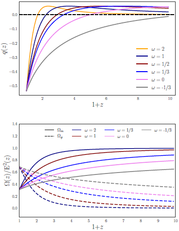
Fig. 1 Deceleration parameter and density fractions vs. redshift, (respectively, on the top and bottom panels), in the presence of a scalar field ϕ. The top panel shows the trend followed by the deceleration parameter q(z) with different effective equations of state ω associated with the cosmic fluid. The horizontal dashed line represents q(z) = 0; below that, the Universe experiences an accelerated expansion. On the bottom panel, we display the density fractions for matter Ω _m (solid lines) and the scalar field Ω _ϕ (dashed lines) for different equations of state of the effective cosmic fluid. Today’s energy fractions, Ω _m,o and Ω _ϕ,o , have been set to ^{Planck Collaboration et al. (2020)} cosmology. The color figure can be viewed online. 

The top panel of Figure 1 reveals interesting insights into the dynamics of the Universe under the presence of the scalar field: only values of ω larger than 1/2 have a transition from matter to the DeSitter-dominated Universe (accelerated expansion of the Universe). Smaller values of the effective equation of state either have a very early turnover from one domination era to the other, or the Universe is always subjected to a cosmic accelerated expansion under the influence of this field.

On the other hand, the bottom panel of Figure 1 displays the evolution of the normalized energy density fractions for matter (solid lines) and the scalar field (dashed lines) as a function of the cosmic fluid equation of state ω. All cases confirm that energy is being released from the field to matter through diffusion. Values of ω smaller than −1/3 (grey line) do not present diffusion from the scalar field to the cosmic fluid, so we leave them aside from this analysis. Finally, it is worth noting that neither of these plots directly depends on the value of σ _o . Instead, the strong dependence lies on ω, which also determines the evolution of the diffusion coefficient σ, according to equation (17).

Figure 2 shows different trends for the diffusion coefficient σ(z) with redshift, with an increasing value of σo=9Ho3⋅Ωm,o⋅Ωϕ,o8πGno from top to bottom. As expected, Figure 2 shows that large values of σ _o lead to a prompter energy release from the scalar field through diffusion. We emphasize that the physical mechanism by which the energy is exchanged between the field and galaxy flow is outside this paper’s scope. Nonetheless, the trends in Figure 2 indicate that diffusion in this model occurs continuously and not as a sudden (instantaneous) event.

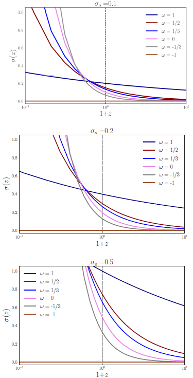
Fig. 2 Diffusion coefficient σ as a function of the redshift, when a scalar field ϕ is imposed in Einstein’s field equations to be the source of the diffusion. We include a brown line representing the ΛCDM model in which diffusion does not occur at any point during cosmic history (σ = 0). The black dashed line indicates the present (i.e., z = 0). Cases with σ _o = 0.1, 0.2, and 0.5 are displayed in the upper, center, and lower panels, respectively. The color figure can be viewed online. 

To conclude this section, we perform a sanity check. Given an equation of state that is exactly −1, no diffusion occurs. The accelerated expansion is due to the dynamics of the field -and a possible link to Λ- rather than a diffusive process driven by ϕ itself.

4. DIFFUSIVE PROCESSES DRIVEN BY A PERFECT FLUID

In this section, we study a different type of solution of the Einstein equations that consider a term ϕg _µν on the left-hand side of the equation (2). Instead, we introduce a perfect fluid with a barotropic equation of state p _D = ω _D ρ _D (we use the subscript D to identify this fluid, which is driving the diffusion).

In this case, the energy-momentum tensor is given by:

With this choice of Tμν', the solutions of the Einstein equations are:

The latter equations lead to the relations:

In addition to the Friedmann equations above, we present a modified version of the continuity equation that comes from eq. (4):

The right term of equation (22) is positive (negative) for matter (diffusive) fluid. As before, we define the density fraction of the diffusive fluid Ω _D as:

Re-writing the derivatives in terms of the redshift z in eq. (22) and setting the system of first-order differential equations from (23) and (22) with the density fractions Ω _m and Ω _D , we obtain:

We stress that the system of differential equations in (24) satisfies the Bianchi identity and introduces an additional perfect fluid in the momentum-energy tensor in eq. (4). As discussed by ^{Calogero (2011)}, one can add an extra term in the stress tensor T _µν on the right-hand side of Einstein’s field equations and re-interpret the inclusion of the scalar field in the geometry side (see § 3).

4.2. Solutions with a Variable Diffusion Coefficient σ

Now, if we allow σ to have evolution with redshift, the solution of the set of differential equations (24) is given by:

Ωm(z)=Ωm,o(1+z)3+3ωDΩD,o, (29a)

ΩD(z)=ΩD,o(1+z)3+3ωDΩD,o. (29b)

On the other hand, the diffusion coefficient is described by the following relation:

σ(z)=ωD(-9Ho3⋅Ωm,o⋅ΩD,o8πGno)(1+z)(3/2+9/2ωDΩD,o), (30)

=σo(1+z)(3/2+9/2ωDΩD,o). (31)

with:

σo=-ωD(9Ho3⋅Ωm,o⋅ΩD,o8πGno). (32)

Equation (32) reveals that ω _D must be strictly negative such that σ > 0, and diffusion is a feasible process. Figure 3 shows the resulting evolution of the Universe with the solutions of the density fractions presented in eq. (29) and the condition found for ω _D .

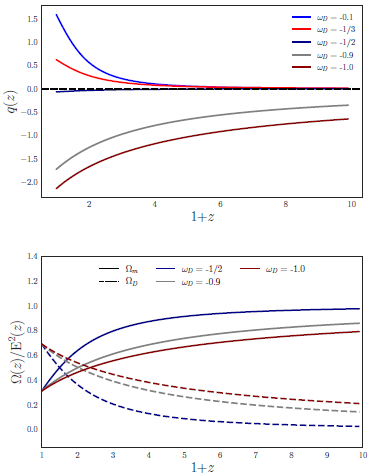
Fig. 3 Deceleration parameter and density fractions vs. redshift, respectively, on the top and bottom panels, in the presence of a perfect fluid with a barotropic equation of state p = ω _D ρ. On the top, we show the deceleration parameter q(z) with different values for equations of state ω _D , such that ω _D < 0, therefore σ is strictly positive. The horizontal dashed line represents q(z) = 0; below that, the Universe experiences an accelerated expansion. On the bottom panel, we display the density fractions for matter Ω _m (solid lines) and the perfect fluid Ω _D (dashed lines) for different equations of state that lead to a negative deceleration parameter. As before, we assume ^{Planck Collaboration et al. (2020)} cosmological parameters for the density fractions at z = 0. The color figure can be viewed online. 

One can notice from Figure 3 that not every negative value of ω _D would lead to an accelerated expansion of the Universe. Values of ω _D greater than −1/2 conduct to a positive deceleration parameter; hence, introducing a diffusive fluid does not cause the effect we are looking for. We rule out these solutions in the rest of the analysis.

However, we also highlight that solutions with ω _D < −1/2 lead to an accelerated expansion in all the redshift range considered. The latter is a consequence of the solutions of eq. (29) not depending explicitly on the diffusion coefficient but on the equation of state of the diffusive fluid.

The bottom panel of Figure 3 shows the evolution of the density fraction only for the values of ω _D that lead to an accelerated expansion of the Universe, i.e., equations of state that are smaller than −1/2.

Figure 4 presents the behavior of the diffusion coefficient as a function of redshift for different values of σ _o .

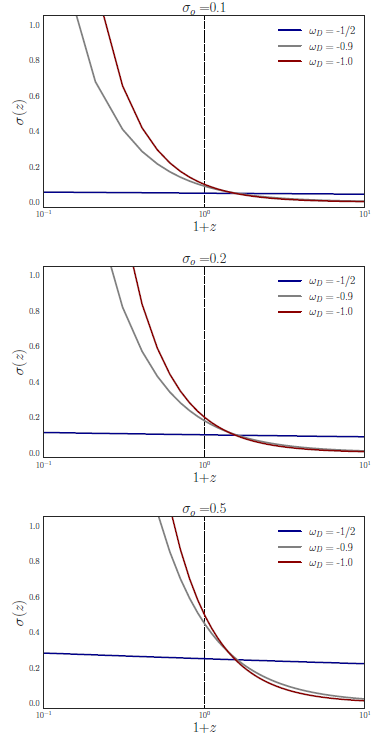
Fig. 4 Diffusion coefficient σ as a function of the redshift, in the presence of a diffusive perfect fluid. The black dashed line indicates the present (i.e., z = 0). Cases with σ _o = 0.1, 0.2, and 0.5 are shown from top to bottom. Regardless of the value of σ _o , ω _D ≈−1/2 leads to a constant diffusion coefficient, exactly the prediction made in equation (27). The color figure can be viewed online. 

It is worth noting that a particular value of ω _D leads to a σ(z) = σ _o , as seen in the blue lines in Figure 4. This specific value is determined by eq. (27), i.e., a diffusive perfect fluid with a constant coefficient.

4.3. Solution for Diffusive Processes with σ=σ-oE(z)

This subsection assumes that the diffusion coefficient is proportional to the function E(z). We remind the reader that H(z) = H _o E(z), and H _o is the Hubble constant that can be measured with different cosmological proxies.

When diffusion occurs in physical scenarios, it is customary to assume that the diffusion coefficient is proportional to the density of the solute. However, the cosmological case is much more complex; thus, it is perfectly natural to explore a case where σ depends on the density fraction of both the solute Ω _m and the solvent Ω _D . A function that relates both densities is E(z). With this choice for σ(z), the set of differential equations (24) are decoupled and its solution is given by:

Ωm(z)=Ωm,o(1+z)3-8πGnoσ-o3Ho3(1+z)3ln⁡(1+z),ΩD(z)=(ΩD,o+8πGnoσ-o9Ho3ωD)(1+z)3(1+ωD)-8πGnoσ-o9Ho3ωD(1+z)3.

Rearranging the terms, it is easy to see that our solutions could be interpreted as a perturbative term on σ _o to the background solutions in a generic dark energy model ωCDM.

Ωm(z)=Ωm,o(1+z)3-σo(1+z)3ln⁡(1+z), (33)

ΩD(z)=ΩD,o(1+z)3(1+ωD)+σoωD((1+z)3(1+ωD)-(1+z)3). (34)

Notice that if σ _o → 0, we recover the density frac ⁱ tions for non-interactive fluids: Ω _i ∝ (1 + z) ^{3(1+ω )} . Another striking point of this set of solutions is that they do not impose any constraint on the parameters ω _D and σ _o .

Figure 5 shows the deceleration parameter as a function of redshift for different values of ω _D and σ _o (from top to bottom).

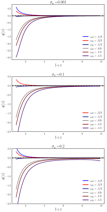
Fig. 5 Deceleration parameter as a function of redshift, when a diffusive fluid is imposed on the energymomentum tensor. The horizontal dashed line represents q(z) = 0; below that, the Universe experiences an accelerated expansion. Although there are no mathematical restrictions on the values for ω _D , values greater than −1/2 lead to a positive deceleration parameter, independent of the value of σ _o . We assume ^{Planck Collaboration et al. (2020)} cosmological parameters for the density fractions at z = 0. The color figure can be viewed online. 

Due to the nature of these solutions and the explicit dependence of the density fractions (therefore, the deceleration parameter) on σ, there is an unexpected outcome that needs further investigation: values of σ(z) larger than 0.25 exhibit a very sharp (discontinuous) transition from a negative to a positive deceleration parameter q(z). This trend can be anticipated with the inflection of the indigo line at high redshift (ω _D = −1/2) in the lower panel of Figure 5.

Finally, we show the density fractions of both matter and diffusive fluids as a function of redshift in Figure 6.

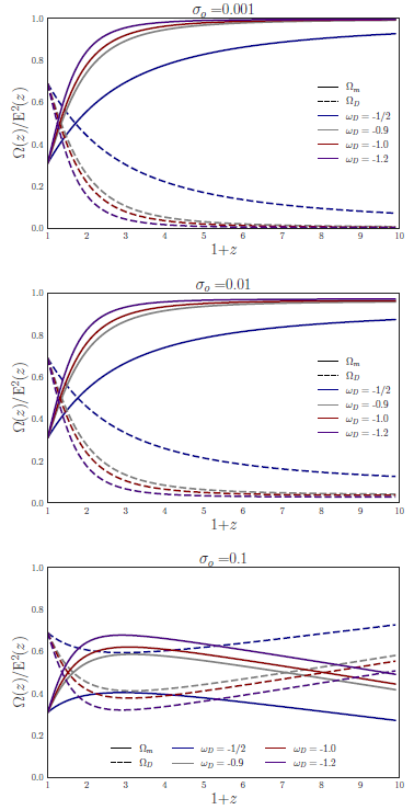
Fig. 6 Density fractions vs. redshift when a perfect fluid with a barotropic equation of state p = ω _D ρ is introduced as a diffusion source. The matter and diffusive fluid density fractions are presented in solid and dashed lines. Notably, the diffusion coefficient can be used as a perturbative parameter in this set of solutions. Therefore, we display the evolution of the density fractions with increasing values of σ in descending panels. We have assumed ^{Planck Collaboration et al. (2020)} cosmological parameters for today’s density fractions. The color figure can be viewed online. 

The perturbative nature of these solutions is exhibited in Figure 6. When σ _o is small (0.001; upper panel), the density fractions look alike to the cosmic scenario with non-interactive fluids. This is also true in the middle panel when σ _o increases by one order of magnitude over the previous σ, but it is still smaller than Ω _m,o by a factor of ≈ 1/30. Nevertheless, if σ _o and Ω _m,o are of the same order of magnitude (lower panel), the energy transfer from the diffusive fluid to the matter component is much more complex, and the process does not follow the order of the domination eras as known: first the matter domination-epoch, and subsequently, when the diffusive fluid overcomes the matter density fraction, a stage of accelerated expansion of the Universe occurs.

5. DISCUSSION AND CONCLUSIONS

In this work, different scenarios for diffusion have been explored, one driven by a scalar field ϕ(t), but also with a perfect fluid with a barotropic equation of state, with ω _D . The former case has been extensively covered by ^{Calogero (2011}, ²⁰¹²⁾; ^{Calogero et al. (2013)}; ^{Velten et al. (2014)}; ^{Alho et al. (2015)}, and their results were used as our primary comparison of the solutions presented in § 3.

As opposed to ^{Calogero et al. (2013)}, we establish exact expressions for the density fractions of the cosmic fluid and the scalar field as a function of redshift, and the effective equation of state ω of the background fluid. We also present two proposals for the evolution of the diffusion coefficient that mostly depend on today’s density fractions and the equation of state ω: constant or redshift-dependent. In the latter case, ω is a free parameter of our theoretical model. Still, effective values of ω ≳ 1 reproduce a smooth transition from a positive to a negative deceleration parameter at z ≈ 1 (the most likely scenario according to a large set of observations).

The second part of the document is devoted to a diffusive perfect fluid that is included in the energy momentum tensor. This fluid is not only stressfree (perfect fluid condition), but also there is a barotropic equation of state p = ω _D ρ that defines its evolution. This is a completely original treatment for diffusion that could explain the Universe’s accelerated expansion at late times.

Three cases are considered for the diffusion coefficient: a constant value, redshift dependent, or proportional to the normalized Hubble parameter E(z).

With this assumption for σ, we find the solutions for the density fractions Ω _m (matter) and Ω _D (diffusive fluid), as well as the restrictions for ω _D .

Our main findings are summarized as follows:

This work offers a new perspective to explain the Universe’s accelerated expansion at late times through diffusion, either caused by a scalar field ϕ or by a perfect barotropic fluid. But as any novel model it is not free of open questions and caveats that need to be addressed in future investigations.

One limitation of our model is that it does not consider the internal structure of galaxies, and all collapsed systems are assumed to have the same mass as in a classical statistical distribution. Also, we adopt a description of galaxies as particles in the solute and neglect any feedback with the intergalactic medium. All of the above could be correct at large cosmological scales but could not hold at the galaxy groups level.

In line with the previous caveat, we highlight that we only consider the Hubble flow, and peculiar velocities are not examined. If perturbations to the FLRW metric are calculated, transverse velocities should change the diffusion scheme presented here.

Our solutions are also restricted to the ^{Planck Collaboration et al. (2020)} cosmological parameters. However, there is no reason to assume the values of the energy fractions of the fields today have to match the ones in Planck cosmology. The next step for this work will be to calculate the free parameters of our model with the large set of cosmological proxies that are publicly available and provide an estimate for the Hubble constant H _o . Thus, we will be able to comment on the Hubble tension, and also set constraints on the diffusion coefficient σ.

The most pressing matter is that diffusive processes are still incompletely formulated in curved space-time. This theoretical diffusion scheme is a macroscopic effective description built on our limited knowledge of the energy transfer processes from the solvent to the solute. Needless to say, this is an extremely challenging problem at a microscopic level in general relativity.

On the other hand, if one could propose an experiment to quantify the value of σ, then it would be possible to rule out from the scenario the existence of the scalar field ϕ, or the perfect fluid with the equation of state ω _D . Even if we set upper limits for the value of σ, we could formulate experiments to estimate the effects of this solvent at a perturbative level.

Assuming that the solvent is a scalar field ϕ, introduced in the field equations in the same way as the cosmological constant Λ, does this mean that the field has finite energy to deliver to the matter field? If so, what will eventually occur when the diffusion mechanism suddenly stops?

This phenomenological model is based on the assumption that a diffusive solvent exists, but what is the nature and origin of such an agent? Is there another fundamental interaction experienced by the solvent (scalar field or perfect fluid) one can use to study its physical properties?