69 5Structural, mechanical, electronic, thermal, and optical properties of the inverse-Heusler compounds X2RuPb(X = La, Sc): A first-principles investigation 
Home Page  

  • SciELO

  • SciELO


Revista mexicana de física

 ISSN 0035-001X

Rev. mex. fis. vol.69 no.5 México sep./oct. 2023   28--2024

https://doi.org/10.31349/revmexfis.69.050401 

Atomic and Molecular Physics

Exact Green’s functions for localized irreversible potentials

J. I. Castro-Alatorre1 

D. Condado1 

E. Sadurní1 

1 Instituto de Física, Benemérita Universidad Autónoma de Puebla, Apartado Postal J-48, 72570 Puebla, México.


Abstract

We study the quantum-mechanical problem of scattering caused by a localized obstacle that breaks spatial and temporal reversibility. Accordingly, we follow Maxwell’s prescription to achieve a violation of the second law of thermodynamics by means of a momentum-dependent interaction in the Hamiltonian, resulting in what is known as Maxwell’s demon. We obtain the energy-dependent Green’s function analytically, as well as its meromorphic structure. The poles lead directly to the solution of the evolution problem, in the spirit of M. Moshinsky’s work in the 1950s. Symmetric initial conditions are evolved in this way, showing important differences between classical and wave-like irreversibility in terms of collapses and revivals of wave packets. Our setting can be generalized to other wave operators, e.g. electromagnetic cavities in a classical regime.

Keywords: Point-like interactions; Maxwell’s demon; Green’s functions

1. Introduction

Explicit time-dependent solutions of the Schrödinger equation have been of interest since the advent of quantum mechanics. In 1952, M. Moshinsky showed [1] that the evolution of a particle beam emerging from a shutter displays important details inherent to interference effects. In the same decade, this study was linked to the poles of the S matrix [2] in scattering theory, including irreversible problems e.g. resonances and nuclear decay [3]. Since then, nuclear, atomic and molecular beams have been used to demonstrate diffraction and quantum interference; in our days, matter waves are best realized by Bose-Einstein condensates [4-7].

In this article, we study a closed dynamical system with spatial and temporal irreversibility, using similar techniques but in a modern context: The microscopic test of the second law of thermodynamics. Our closed system consists of an arbitrarily large ensemble of independent particles described by the Schödinger equation under the influence of a momentum-dependent potential localized in some small region - an obstacle. In the classical regime, the so-called Maxwell’s demon [8] falls into this class of problems, whereby the process of discriminating particles by their velocity is called Maxwellian irreversibility. With this in mind, it is possible to study the quantum effects of an interaction potential that depends on the momentum of a wave, i.e. an operator that addresses its Fourier component. Such momentum-dependent interactions have been used extensively to model nuclear, molecular or even relativistic dynamics [9-11]. Thus, we expect that a point-like defect that operates on a particle according to its velocity, should reproduce reasonably well the classical division of fast and slow components of an ensemble into two compartments, plus interference effects that we shall discuss carefully in our treatment.

The mathematical goal of this work is to obtain in closed form the corresponding energy-dependent Green’s function, thus providing an analytical solution to scattering and time-dependent evolution via Laplace inversion. It should be noted that such a function will have broken exchange symmetry (e.g., G(x,x')G(x',x)), as is to be expected for a system with Maxwellian irreversibility or broken time reversal invariance. Explicit Green’s functions with such properties are scarce in the literature [12, 13], so our results shall include new formulae for these objects.

In terms of applications, the limitations of the second-law of thermodynamics have been discussed since the appearance of Maxwell’s demon [14-21], but they have not been emulated dynamically so far in the quantum realm; instead, informational treatments have been used which, in general, are based on measurements and feedback [14-21] in various types of arrangements, such as photonic setups [27, 28], ultracold atoms [29], superconducting quantum circuits [30], QED cavities [31], quantum dots [32] and electronic circuits [33, 34]. In view of this, our approach shall be ideal for applications that involve wave dynamics of a broader type, without wave collapse mechanisms; electromagnetic cavities can be considered if one perturbs the Helmholtz operator with complex terms, as in dielectric media.

In Sec. 2 we introduce a momentum-dependent potential in a classical Hamiltonian that exerts Maxwellian irreversibility on the particles involved, and then we generalize it to the quantum mechanical domain. Subsequently, the formalism of irreversible non-symmetric Green’s functions is introduced, obtaining thereby a new closed expression. Lastly, in Sec. 3 we present a dynamical analysis of symmetric initial conditions.

2. Maxwellian Irreversible Problems with Localized Interactions

We motivate our discussion with a classical problem that consists of an ensemble of particles in an origin-centered container with a length of 2xL. In this context, particles are considered independent, therefore the action of a potential is separable and a Hamiltonian formulation per particle is possible. For this system, the Hamiltonian takes the form

H=p22m+Vbox(x)+Vint(x,p), (1)

where V box represents a pair of impenetrable barriers at x=±xL, V int is a momentum-dependent potential with strength V 0 at x = 0, i.e.,

Vint(x,p)=V0δ(x)Vact(p), (2)

and Vact(p) is an activation function that determines whether particles remain on one side of the container or pass to the other side according to the particle’s momentum. In particular, we have the following expression

Vact(p)=f-(|p|)sgn(p)+f+(|p|), (3)

with

2f±(|p|)=Θ(PR-|p|)±Θ(|p|-PR)Θ(|p|-PUV), (4)

where the reference momentum P R will discern which particles will be influenced by the perturbation, depending on their momentum, whereas the δ distribution is a contact interaction depending on particle’s position. In addition, an ultraviolet cutoff P UV can be introduced in case the potential does not operate at high frequencies; for instance, in electromagnetic realizations P UV is necessary, as dielectric materials operate in specific ranges (see Fig. 1).

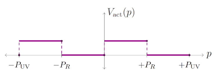
Figure 1 Activation potential V act(p) defined in (3) with reference momentum P R and ultraviolet cleaving P UV

To appreciate the effect of this potential, suppose two ensembles ρ 1 and ρ 2, shown in Fig. 2: ρ 1 represents a collection of independent particles in the first quadrant with a right-directed momentum less than P R , therefore, when the system evolves, the phase space corresponding to the zone -xL<x<0 and |p|<|PR| will be filled. Conversely, ρ 2 represents a collection of independent particles in the third quadrant with a left-directed momentum greater than P R , so, when the system evolves, the phase space corresponding to the zone 0<x<xL and |p|>|PR| will be filled. It should also be noted that, after the selection process has taken place, the system reaches an equilibrium where each compartment possesses temperatures T 1,2 such that

T2(x>0)>T1(x<0). (5)

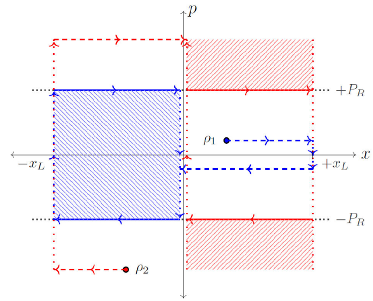
Figure 2 Phase space evolution of two particle ensembles ρ1(|p|<|PR|) & ρ2(|p|>|PR|). The activation potential separates particles according to the reference momentum, leaving two well differentiated zones. 

Therefore V act(p) effectively separates the particles into two well differentiated zones according to their momentum.

2.1. Quantum mechanical generalization

Now we can omit the presence of V box in the Hamiltonian operator by introducing Dirichlet boundaries. It is also important to preserve the hermiticity of H by defining properly the irreversible potential. To this end, we first promote Vint(x,p) in (2) to an operator

V^int(x^,p^)V0δ(x^)V^act(p^), (6)

which must be symmetrized in order to get a hermitian potential. First, we note that the action of V^act(p^) on a complete basis of plane waves is V^act(p^)exp(ikx)=Vact(k)exp(ikx), where Vact(k) is just a number as specified by the classical function (3). Therefore, the action of (6) on any wave given by ψ(x)=x|ψ can be defined by means of the action of V^act(p^) on the state |ψ 〉; we have

V^act(-i)x|ψ=xV^act(p^)ψ=-dpxV^act(p^)pp|ψ=-dpVact(p)x|pp|ψ=-dp -dx'Vact(p)x|pp|x'x'|ψ=-dx'-dpVact(p)eip(x-x')/2πx'|ψ=-dx'V~act(x'-x)ψ(x'), (7)

where V~act is the Fourier transform of Vact. This procedure is valid even for Dirichlet boundaries, as 𝜓 above may have compact support and its Fourier integral will be reduced to the domain -xL<x'<xL. The symmetrization of the operator (6) is the following hermitian potential V^=(1/2)(V^int+V^int), and it renders the Schrödinger equation as

-22m2Ψx,t+V02δx^V^(-i)+V^-iδ(x^)Ψ(x,t)=itΨx,t. (8)

The goal is to solve (8) using energy-dependent Green’s functions. We emphasize that the explicit form of the eigenfunctions is not necessary to obtain the spectral decomposition of Green’s functions in closed form. An example of this can be seen in Appendix A, where the Green’s function for a δ(x)-potential is calculated solely using the integrals in the Lippmann-Schwinger equation.

2.2. A Theorem on Non-Symmetric Green’s Functions

It is known that Green’s functions are not always symmetric: the cases in which symmetry under exchange of spatial variables is recovered correspond to real Hamiltonians and time-reversibility. To see this, we present the following elementary theorem:

Theorem. LetG^(±)be a solution of(H^-E)G^(±)=I and G^(±)(H^-E)=I, whereH^is Hermitian and G^(±)in the position-basis is 〈x|G^(±)|x'〉=limε0+〈x|1/H^-Eiε|x'〉=G(±)(x,x';E). Then(G(±)(x,x';E))*=G()(x',x;E)).

Proof. In the position-basis,G^(±)must fulfill

Hx,-ix-EG(±)x,x';E=δx-x' (9a)

and

H*x',-ix'-EG(±)x,x';E=δx-x'. (9b)

Taking a Hamiltonian such thatH=H, it follows that

G^(±)=G^(), (10a)

or, expressed in the position basis

xG^(±)x'=xG^()x'. (10b)

Note that the left-hand side becomes

xG^(±)x'=(x'G^(±)x)*

after taking out the conjugate transpose. Consequently,

G(±)x',x;E*=G()x,x';E. (11)

So the advanced and retarded Green’s function, for this case, are related to an index exchange and complex conjugation.

Corollary G(±)(x,x';E) is symmetric if and only if the Hamiltonian is real.

Proof. ⇒) By taking a Hamiltonian such that H = H * , it follows that

G^(±)*=G^() (12a)

or, expressed in the position basis

xG^(±)*x'=xG^()x'. (12b)

Note that the left-hand side can be transformed into

x((G^(±)*)T)Tx'=x(G^(±))Tx'=x(G^())Tx',

where (10a) was used in the last step. Consequently,

x'(G^())x=xG^()x'. (13)

Therefore,G(±)(x,x';E)is symmetric.

⇐) Suppose that

G(±)(x,x';E)=G(±)(x',x;E), (14a)

or, expressed in Dirac notation

xG^(±)x'=x'G^(±)x. (14b)

Note that the right-hand side can be transformed into

x'(G^(±))x=x'G^()x=xG^()*x'

where (10a) was used in the middle step. Consequently,

xG^(±)x'=xG^()*x'. (15)

Therefore,G^(±)*=G^(), and the Hamiltonian is real.

2.3. Exact form of Green’s function

Now we focus on the analysis of a function G Demon that solves the following problem

H+V(x,p)-EGDemon=δx-x', (16)

where H is any Hamiltonian whose Green’s function G 0 is known and V(x, p) is the Maxwellian interaction in (8). From here on we work with units =1. We recall that a particle with a Dirac-delta potential gives rise to an equation with a source, similar to the Lippmann-Schwinger equation. This allows an exact solution for the energy-dependent Green’s function by an evaluation of the corresponding integrals in the first term of the Born series. Note however that when the potential is affected by a momentum-dependent activation function (hence irreversible), the integral is more involved, as G is self-contained in the expressions. For this reason, we must address an integral equation as well as a functional relation. The explicit equation in operator-form to be solved is

H^-E+V(p^)δ(x^)+δ(x^)V(p^)G^p=I. (17)

Inspired by the solution of a delta perturbation that depends only on position (see Appendix A), the following integral equation is obtained

Gp(x,x',E)=G0(x,x',E)-dy G0(x,y,E)δ(y)V(p^)Gp(y,x',E)-dy G0(x,y,E)V(p^)δ(y)Gp(y,x',E), (18)

where the momentum operator p^ in the expression above is understood as -iy. Prior to the evaluation of (18) we insert another complete set in each integral in the form

yδ(x^)V(p^)G^px'=dy' yδ(x^)V(p^)y'y'G^px'=dy' δ(y)2πdp eip(y-y')V(p)Gp(y',x',E)=δ(y)dy' V~(y')Gp(y',x',E), (19a)

where a complete set of plane waves was introduced in the second line, and as before

V~(y')=12πdp e-ipy'V(p), (19b)

is the Fourier transform of the potential; whereas, for the second integral, we have

yV(p^)δ(x^)G^px'=dy' yV(p^)δ(x^)y'y'G^px'=dy' δ(y')2πdp eip(y-y')V(p)Gp(y',x',E)=V~(-y)dy' δ(y')Gp(y',x',E)=V~(-y)Gp(0,x',E). (19c)

Substitution of (19) in (18), leads to

Gp(x,x',E)=G0(x,x',E)-G0(x,0,E)dy' V~(y')Gp(y',x',E)-dy G0(x,y,E)V~(-y)Gp(0,x',E). (20)

In order to get Gp(x,x',E), we first multiply the last expression by V~(x) and integrate over x,

dx V~(x)Gp(x,x',E)=dx V~(x)G0(x,x',E)-dx V~(x)G0(x,0,E)dy' V~(y')Gp(y',x',E)-dx V~(x)dy G0(x,y,E)V~(-y)Gp(0,x',E), (21)

and recognizing that the integral on the left-hand side is the same as the one in the 2nd term of the right-hand side (with another integration variable), a consistency condition is obtained:

dy' V~(y')Gp(y',x',E)=P1(x',E)-Q1(E)Gp(0,x',E)1+Q2(E), (22)

where

P1(x',E)=dx V~(x)G0(x,x',E), (23a)

P2(x,E)=dy G0(x,y,E)V~(-y), (23b)

Q1(E)=dx dy V~(x)G0(x,y,E)V~(-y), (23c)

Q2(E)=dx V~(x)G0(x,0,E). (23d)

Substituting the above equation again into Gp(x,x',E) given by (18), leads to the following functional equation

Gp(x,x',E)=G0(x,x',E)-P2(x,E)Gp(0,x',E)-G0(x,0,E)P1(x',E)-Q1(E)Gp(0,x',E)1+Q2(E). (24)

The latter is not yet a closed formula for G p , for it depends on G p again. Evaluating at x = 0 provides the reduced functional equation

Gp(0,x',E)=G0(0,x',E)-P2(0,E)Gp(0,x',E)-G0(0,0,E)P1(x',E)-Q1(E)Gp(0,x',E)1+Q2(E), (25)

which can be solved for Gp(0,x',E), leaving

Gp(0,x',E)=G0(0,x',E)-G0(0,0,E)R1(x',E)1+P2(0,E)-G0(0,0,E)Q3(E), (26a)

where

R1(x',E)=P1(x',E)1+Q2(E),Q3(E)=Q1(E)1+Q2(E). (26b)

The last equation is substituted into Gp(x,x',E), to obtain its final expression in terms of G0(x,x',E)

Gp(x,x',E)=G0(x,x',E)+G0(x,0,E)G0(0,x',E)Q3(E)1+P2(0,E)-G0(0,0,E)Q3(E)-G0(x,0,E)R1(x',E)1+P2(0,E)1+P2(0,E)-G0(0,0,E)Q3(E)-P2(x,E)G0(0,x',E)-G0(0,0,E)R1(x',E)1+P2(0,E)-G0(0,0,E)Q3(E). (27)

This is a new formula for our Green’s function. We shall see that (27) can be split into symmetric and antisymmetric contributions, where the latter are associated with irreversibility, as we have seen from the theorem in the previous section.

3. Application to a particle in a container

We now specialize in the case where particles are in a container with Dirichlet boundary conditions. The Green’s function and the energies are well known for the unperturbed problem. Our plan is as follows: first we apply our new Green’s function formula to the case of the container with an irreversible perturbation inside; we give the explicit form of its spectral decomposition, and we analyze its meromorphic structure in order to find its poles. Subsequently, we focus on the evolution problem; therefore, we shall need an appropriate definition of entropy that accounts for the emergence of disorder in energy space. To this end, a basis-dependent entropy is suggested. The next subsection is devoted to the use of Shannon’s entropy in our evolution problem. Afterwards, we address the explicit problem of numerical evolution by means of spectral decomposition and a finite-difference method in space. Efficient numerical evaluations are best achieved if this discretization is restricted to a region where the dispersion relation is well approximated by a parabola. Thus, we include a careful analysis of the dispersion relation in the spatially-discretized version of the problem. Lastly, we construct specific initial conditions that are completely symmetric and analyze how the wave packet propagates inside the container asymmetrically. The reason is obviously the inherent broken spatial symmetry of the problem, i.e., the transformation x → -x, p → -p is not a symmetry of H. Then we add a special definition of temperature (or effective beta parameter). Therewith we can analyze other types of time-evolving distributions. In this part, it is important to show how the entropy can indeed decrease as a function of time, resulting in a special kind of ordering or sorting of fast and slow particles, produced by the non-reversible Maxwellian potential.

We start with a free Green’s function in a container G0C, i.e.,

G0C(x,x',E)=2Lm=1sin(κ2mx)sin(κ2mx')E2m-E+2Lm=1cos(κ2m-1x)cos(κ2m-1x')E2m-1-E (28)

with κn=nπ/L and eigenenergies En=(1/2)2κn2. Although this problem does not have asymptotic states, the perturbed system can be regarded as a scattering problem for waves inside the box. It is important to clarify that our approach using plane waves in (7) is still valid here. One may as well resort to a basis of box functions for this purpose, but computations would be more involved. Now let us employ our new result: The Green’s function (28) can be put in terms of Jacobi’s theta function as reported by [12]. The Green’s function in (27) with the container is

GpC(x,x',E)=G0C(x,x',E)+P1C(x,E)G0C(0,x',E)-G0C(x,0,E)P1C(x',E)1-G0C(0,0,E)Q1C(E)+G0C(x,0,E)G0C(0,x',E)Q1C(E)1-G0C(0,0,E)Q1C(E)-P1C(x,E)G0C(0,0,E)P1C(x',E)1-G0C(0,0,E)Q1C(E), (29)

where P1C and Q1C are the integrals evaluated with G0C. From the previous expression the identification of the symmetric and antisymmetric part of the Green’s function is effortless. Note that terms that contribute to the antisymmetric part come from the Maxwellian perturbation, as the first and third terms are manifestly symmetric.

3.1. Pole structure analysis

The integrals in (27) can be done in terms of sine-integral functions [31] (Si) using in addition the Fourier’s transform of the potential described in Fig. 1, e.g.

V~(±y)=±12iπy(1-2cosPRy), (30a)

P1C(x',E)=-P2C(x',E)=-2iπLn=1Si(ξ+)-Si(ξ-)-Si(nπ)E2n-Esin(κ2nx'), (30b)

Q1C(E)=2π2Ln=1Siξ+-Siξ--Sinπ2E2n-E, (30c)

Q2C(E)=0, (30d)

with

ξ±=PR±κ2nL2. (30e)

Given the behavior of the Si function in P1C and Q1C(E), the following approximation can be made. The argument is written as

Si(nπ+a)-Si(nπ-a)π2-π2Θ(n-a/π)+π2Θ(a/π-n)+πϵ δn,a/π. (31)

where a=PRL/2, a/π represents the integer part and 𝜖 the fractional part of a/π and the step function is zero for the case n=a/π. (The full procedure is in Appendix B). So the integrals are now approximated by

P1C(x,E)-2iLn=1a/π-1sin(κ2nx)E2n-E-12n=1sin(κ2nx)E2n-E+12(1+2ϵ)E2a/π-Esin(κ2a/πx), (32a)

and

Q1C(E)12Ln=11E2n-E-1E2a/π-E. (32b)

The pole structure of the whole antisymmetric term can be very intricate. According to the transcendental equation

1-G0C(0,0,E)Q1C(E)=0, (33)

where it is straightforward to see that

G0C(0,0,E)=tan(L2E/2)2E,Q1C(E)=12L12E-Lcot(L2E/2)22E-1E2a/π-E,

and clearly E2a/π is not a zero of (33), since the product G0C(0,0,E)Q1C(E) would tend to infinity if EE2a/π. However, it is noted that the numerator

P1C(x,E)G0C(0,x',E)-G0C(x,0,E)P1C(x',E) (34)

still contains the poles of G0C; while the new term P1C(x,E), proportional to sin(κ2a/πx)/(E2a/π-E), which in general (if xx') does not disappear, contributes to a new pole located at E2a/π. To sum up, the antisymmetry under exchange xx' in both stationary and time-dependent solutions comes predominantly from the harmonic inversion of (34) under the approximation

sin(κ2a/πx)G0C(x',0,E)-G0C(0,x,E)sin(κ2a/πx')E2a/π-E

whose pole produces exp(-iE2a/πt/) in the spectral decomposition of the wave function, and thus a typical frequency.

3.2. Shannon’s Entropy

The entropy is fundamental in the analysis of asymmetric evolution inasmuch a dynamic effect of apparent ordering is sought. Since the von-Neumann equation without a source does not capture the irreversibility phenomenon, a notion of entropy that describes disorder with respect to a specific basis (e.g. energy) is required. Shannon’s definition of entropy is

σSh=-mϱm log ϱm. (35)

where the probabilities ϱm will be given by the overlap (integral) of the wave function with the basis of the free problem, i.e.

ϱm=|m,Em(0)Ψ,t|2=n'm,Em(0)n'n'Ψ,t2. (36)

Likewise, the total entropy of the system must be estimated separately, as Shannon’s entropy applies only to the particles inside the container, but does not contemplate the reaction of V(x,p) itself, which is not dynamically involved. To this end, we estimate the work done by the potential on the trapped wave and vice versa. Also, using the principle of extensivity one can find a lower bound for the total entropy of the system S t as the linear combination of the particle’s entropy S p plus Maxwellian-potential’s entropy S d, i.e.

ΔSt=ΔSp+ΔSd?0 (37a)

with ΔSp0 as the entropy of the particles must decrease because of the Maxwellian potential. Furthermore, one can find a lower bound for the Maxwellian-potential’s entropy change in terms of the work done by the potential as

ΔSd=δ'QT    ΔQT1TΔV=(const.)ΔV. (37b)

From this, it follows that

ΔStΔSp+(const.)ΔV. (37c)

Therefore, when taking into account the work done by the Maxwellian potential, its contribution must compensate for the partial entropy reduction. Indeed, for a container with two separated compartments with volume 𝜐, the change in the particle’s entropy is

ΔSp=-PRTR+PLTLυ log 2, (38a)

where PR,L and TR,L are the pressure and temperature for the right (R) and left (L) compartment, computed as ideal gases. Moreover, the internal energy UPυ, so

ΔSp-βBUR+UL log 2, (38b)

where βB is the thermodynamic beta and UR,L the corresponding lateral internal energy. We shall employ these considerations in the numerical treatment of the problem.

3.3. Spatial and spectral decomposition

We proceed to discretize the Hamiltonian on a lattice. This enable us to treat the problem as a matrix representation on a basis of point-like functions. Since the treatment is equivalent to a tight binding model in a crystal, it is advisable to use the first Brillouin zone to calculate the energies. In this way, the activation potential in (3) will be non-zero in the intervals [-κ D , -κ R ] and [0, κ R ], resulting in the action zones of the Maxwellian potential according to the reference momentum PRκR. This can be seen in the graph below in Fig. 3. However, it is necessary to work in the quasi-parabolic energy regime that is below the Dirac point [36] (ϖD), obtaining the upper graph, a parabola with regions where the Maxwellian potential acts. It is worth mentioning that the region of the potential for p<-PR is not bounded above as in the graph below.

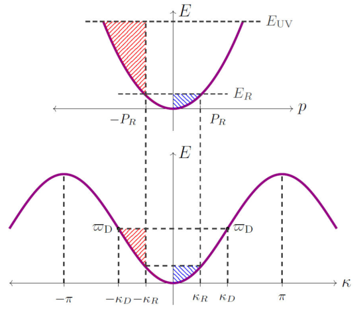
Figure 3 The graph below shows the energies in a tight binding model in a crystal, the coloured zones represent the activation potential in (3) with reference momentum PRκR. Also, using the quasi-parabolic energy regime below the Dirac point(ϖD), the upper graph is obtained. 

Therefore, the Hamiltonian’s action on a plane wave

κ=12πneiκnn, (39)

is no longer restricted to the unperturbed part plus the defect at the origin, instead we have a non-local effect that can be obtained directly by calculating the matrix elements at site n

nHκ=2ma21-cos κeikn2π+12iπn2π2 cos κRn-1-e-iκDn-n'δn,02iπn'eiκn'2π2cosκRn'-1-eiκDn'. (40)

where a is the scale parameter. Also, the Hamiltonian will be diagonalized using a discretized basis n, as many sites as frequencies are necessary, i.e.

nHn'=-22ma2δn-1,n'-2δn,n'+δn+1,n'+V02δn',02iπn2 cosκRn-1-e-iκDn-V02δn,02iπn'2 cosκRn'-1-eiκDn'. (41)

Note that for the central element (the evaluation of the corresponding integrals at n=0=n'),

0H0=22ma22+V02κDπ. (42)

This shows that the potential at its location is finite in a discretized setting, and its intensity V0 can be adjusted at will.

Finally, the wave function Ψ(t) at site n is

nΨ,t=mexp-itEm/nm,Emm,EmΨ0, (43a)

where E m are the eigenvalues of the problem, nm,Em are stationary functions i.e. eigenvectors, while m,EmΨ0 is the overlap (integral) of the initial condition with the basis, i.e.

m,EmΨ0=n'm,Emn'n'Ψ0, (43b)

where n'Ψ0 is the initial condition.

3.4. Dynamical analysis of symmetric initial conditions

The Shannon analogue of a Boltzmann thermal distribution [37] (e.g. as understood by superposition of particle’s number in photonic states) can be used as an appropriate initial condition for box states. The idea is to monitor its evolution and its subsequent ordering. We have:

ψ0B(β,n)=q=1Nmaxexp-βq2-1sinqn+Nπ2N, (44)

here n is the site such that -NnN (the Maxwellian potential is at n = 0), Nmax=2N+1 is the maximum number of q box states that are meaningful in a discretized system, and β is an order parameter which would correspond to

β=E0kBT,    with    E0=π222mL2 (45)

in thermodynamics. This probability overlaps with the components of the eigenvectors νm(n) of (41).

Ψ0B(β,m)=n=12N+1ψ0B(β,n)νm(n)* (46)

obtaining the wave function at the rescaled time τ (=t/2ma2 [adim])

ΨB(β,n,τ)=m=12N+1exp-iτ ΞmΨ0B(β,m)νm(n), (47)

where Ξ (=2ma2E/2 [adim]) are the rescaled eigenenergies of (41).

An example of evolution is shown in Fig. 4. The system size is 2N+1=249 sites, with scale parameter a=L/2N, the rescaled potential intensity is Υ0=(1/10)(=ma2V0/2 [adim]), the reference momentum is κR=π/4 and β=1/100. For relatively short times τ(×10-3)2, a decrease of the entropy in (35) is appreciated. Then, between τ(×10-3)3 to 9 the entropy increases, which is explained by the natural wave expansion in each compartment, to decrease again at τ(×10-3) 12.

Figure 4 Entropy with β=1/100. A decrease of the entropy is seen at τ(×10-3) 2 and 12. 

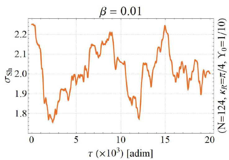
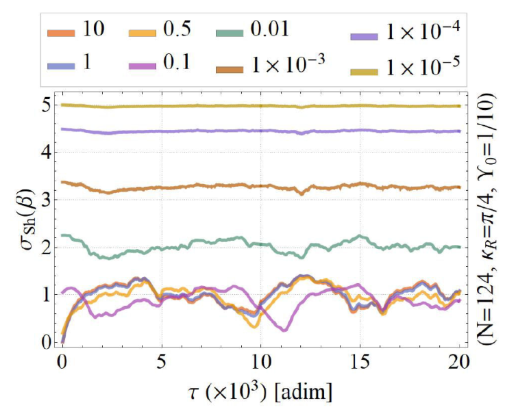
Now we turn our attention to Fig. 5 where we show a comparative plot of entropies by varying the temperature value. It is found that values1/2>β>1/200 produce significant fluctuations for a potential intensity Υ0=1/10. It should be stressed that for higher values of Υ0, the overall behavior shifts to larger values of beta. For very high temperatures, a highly disordered system in the energy basis has a tendency to fluctuate around its original entropic value (quasi-stationary behaviours), this implies that the effect is not strong in these cases. We have found, through these numerical results, that the role played by κR is only partially decisive in the creation of box asymmetries in the evolution, as the intensity Υ0 is also important for small values of beta. However, we must stress that Υ0 cannot be taken as infinite, since all waves would be trapped in such a case.

Figure 5 Comparative plot of entropies by varying the temperature value β

In Fig. 6 we can see asymmetries induced as time elapses, with must drastic effects occurring around τ(×10-3)8.5 where the difference between left and right probabilities (occupation) is large. Note that the effect is recurrent for larger times. In addition, the entropy has a minimum when the probability has a maximal rate of change with respect to time, implying that the Maxwellian potential operates until it reaches a quasi-stationary regime, where there is no exchange of densities but there is entropic rise.

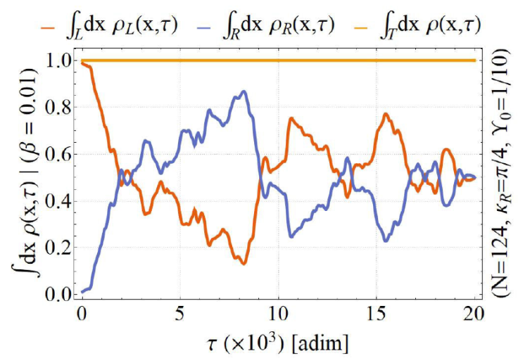
Figure 6 Lateral probabilities for the left (L, red line) and right (R, blue line) part of the container with β=1/100

In Fig. 7 we display lateral averages of the total energy as functions of time. We find asymmetries in both quantities: initially, the thermal wave is biased to the right. Then, between τ(×10-3)= 0 and 5 there is an expansion regime where there is thermalization. For τ(×10-3)>5 the Maxwellian-potential’s action enters the game and the waves are segregated again. These curves are compared with those of Fig. 8, where indeed the average potential energy becomes negative for τ(×10-3)>5, indicating that the particles exert work on the Maxwellian potential (see a global minimum of V at τ(×10-3)9. In this setting, we conclude that our device operates well until the wave expansion allows an important interaction with V at τ(×10-3)=5 and after. For very large times, a regime with noisy collapse-and-revival behaviour can be seen.

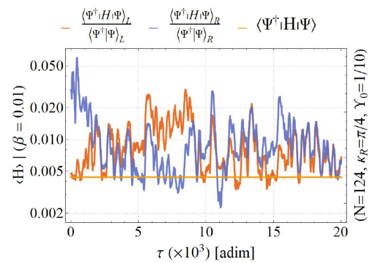
Figure 7 Average internal energy for the left (L, red line) and right (R, blue line) part of the container with β = 1/100. 

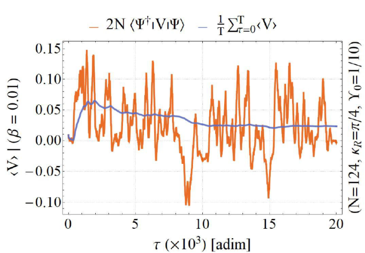
Figure 8 Average Potential Energy. It contributes significantly to the energy balance. The blue line indicates the time average at time τ. Negative values imply work done by the wave on the Maxwellian potential. 

In Fig. 9 we show a density plot for (47). The Talbot effect induces a recurrence time in the quasi-temporal coordinate that will force the system to repeat its behaviour. In this case, τTalbot10(×103), and for τ<τTalbot there is an asymmetry that shows the efficient work of the Maxwellian potential. Subsequently the behaviour is reversed between the compartments of the box.

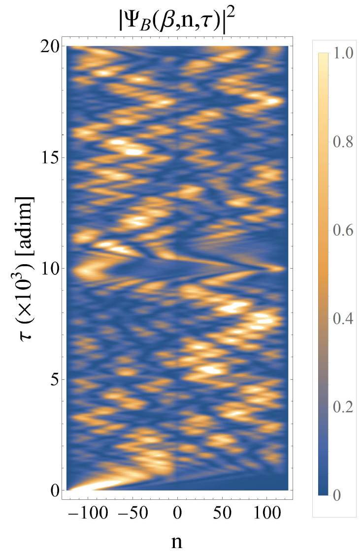
Figure 9 Evolution of a Boltzmann distributed wave packet in the interval -124n124 (horizontal axis) at τ = 0 (vertical axis), interacting with a Maxwellian potential located at n = 0, with β=1/100,  κR=π/4 and Υ0=1/10. The colouration exhibits the probability density, showing that for 5<τ(×10-3)<10 the wave packet is predominantly on the right side. 

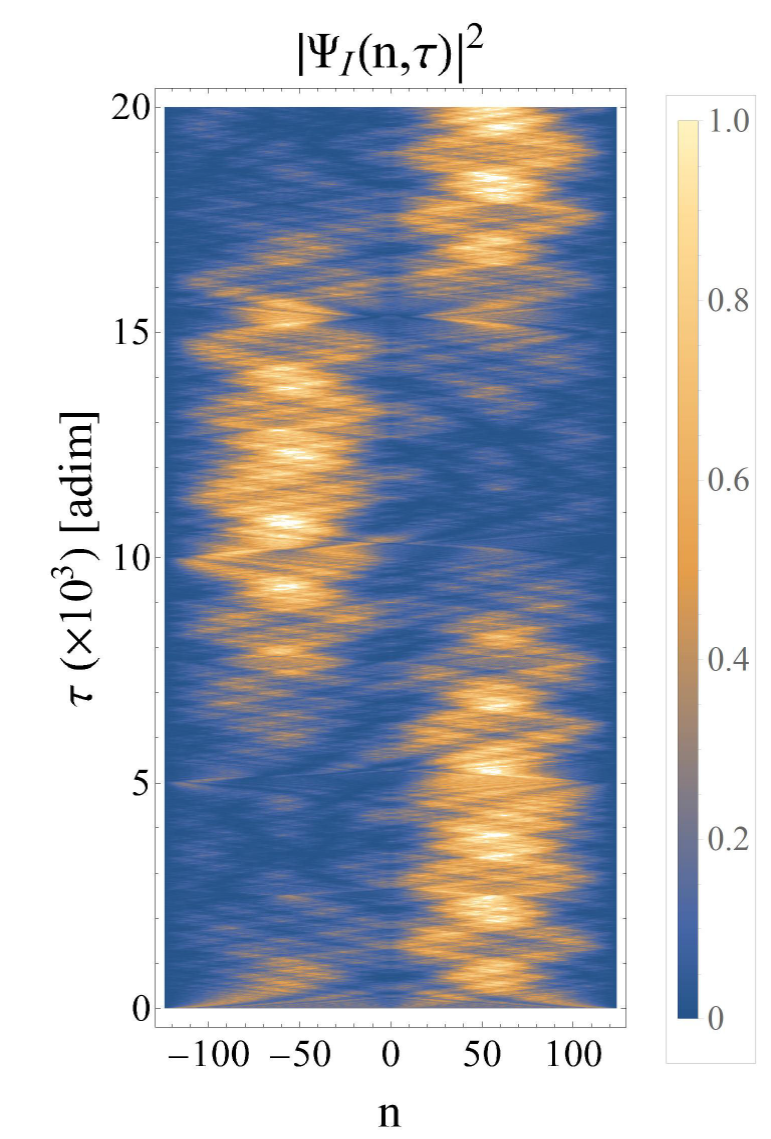
Another situation of interest is the uniform distribution, i.e. Ψ0I=1, (this is denoted by β= IS0). For this case the entropy evolution is shown in Fig. 10. Note that the entropy value oscillates, again reaching a minimum as the system evolves. A density plot of the wave function ΨI(x,τ) shown in Fig. 11, reveals that the wave is distributed asymmetrically due to terms that break parity explicitly as expected.

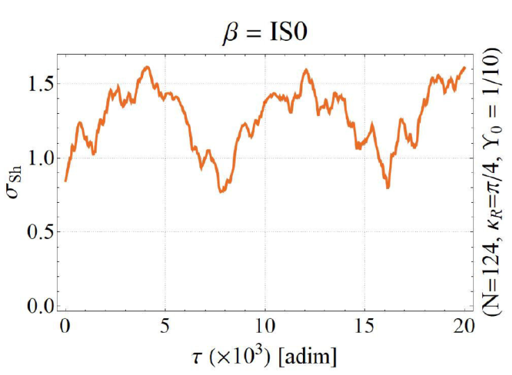
Figure 10 Entropy of an isospectral wave packet. A decrease of the entropy is seen at τ(×10-3) 8 and 16. 

Figure 11 Evolution of an isospectral wave packet in the interval -124 ≤ n ≤ 124 (horizontal axis) at τ = 0 (vertical axis), interacting with a Maxwellian potential located at n = 0, with κ R = π/4 and Υ0 = 1/10. 

4. Conclusions

We have dealt with an irreversible problem in time and space. In particular, we have reported a new asymmetrical Green’s function in closed form pertaining to irreversible systems, not found in standard Refs. [12]. The meromorphic structure of such a solution has been docile enough to allow proper identification of energy ranges where a Maxwellian sorting device is effective. In this way, we have identified how through a Fourier semi-transform the propagator of a real problem will be perturbed due to irreversibility. The symmetry breaking is located in a special term in the Green’s function, whose pole is related with the reference energy at which a demon operates.

Afterwards, a dynamical model for a system that splits an ensemble of waves representing independent particles has been proposed and successfully studied. Our description has been possible via a Hamiltonian operator given by (1) and the irreversible potential in (3). The system works with a reference momentum that decides how two subsystems, with different temperatures, are distributed in each compartment of the cavity. The outcome is reminiscent of the classical demon’s action shown in Fig. 2, as we have confirmed by analyzing wave dynamics in Fig. 9. As an interesting result, the undulatory version of Maxwell’s demon contains -in its evolution- the interference structure of Talbot (quantum) carpets in time domain.

The reader familiarized with Jacobi theta functions may find in our interference patterns the typical trajectories of constant theta value that appear in many other applications, including factorization of natural numbers using Gaussian sums [38]. For long times, a structure of collapses and revivals can be distinguished. This structure displays the expected spatial asymmetries for limited periods of time associated with Talbot lengths. There is no true thermalization (as opposed to the classical process) because of such revivals. A number of quantities and their time behavior support our conclusions in connection with irreversibility and the apparent entropy decrease. Indeed, with Shannon’s definition for a basis-dependent disorder function (in energy states) we observe regimes where ordered configurations are established as time elapses. Also, densities and average energies at each compartment were studied. (Fig. 7 is unmistakable in this respect.) As mentioned in the introduction, our approach to irreversibility can be applied to many types of waves. Particular attention should be paid to electromagnetic cavities, since non-hermitian wave operators with odd space parity emerge naturally in dielectric media. Numerical implementations are left for future work.

References

1. M. Moshinsky, Diffraction in time, Physical Review 88 (1952) 625. [ Links ]

2. M. Moshinsky, Boundary conditions and time-dependent states, Physical Review 84 (1951) 525 . [ Links ]

3. M. Moshinsky, Poles of the S matrix for resonance reactions, Physical Review 91 (1953) 984. [ Links ]

4. K. B. Davis, M. O. Mewes, M. R. Andrews, N. J. van Druten, D. S. Durfee, D. M. Kurn, and W. Ketterle, Bose-Einstein condensation in a gas of sodium atoms, Physical Review Letters 75 (1995) 3969-3973. [ Links ]

5. M. H. Anderson, J. R. Ensher, M. R. Matthews, C. E. Wieman, and E. A. Cornell, Observation of Bose-Einstein condensation in a dilute atomic vapor, Science 269 (1995) 198. [ Links ]

6. M. Meister, A. Roura, E. M. Rasel, and W. P. Schleich, The space atom laser: an isotropic source for ultra-cold atoms in microgravity, New Journal of Physics 21 (2019) 013039. [ Links ]

7. C.-C. Chen, R. G. Escudero, J. Minář, B. Pasquiou, S. Bennetts, and F. Schreck, Continuous Bose-Einstein condensation, Nature 606 (2022) 683. [ Links ]

8. J. C. Maxwell, Theory of Heat (Cambridge University Press, 2009). [ Links ]

9. C. Dorso and J. Randrup, Early recognition of clusters in molecular dynamics, Physics Letters B 301 (1993) 328. [ Links ]

10. P. Cordero and E. S. Hernández, Momentum-dependent potentials: Towards the molecular dynamics of fermionlike classical particles, Physical Review E 51 (1995) 2573. [ Links ]

11. Y. Nara, T. Maruyama, and H. Stoecker, Momentumdependent potential and collective flows within the relativistic quantum molecular dynamics approach based on relativistic mean-field theory, Physical Review C 102 (2020) 024913. [ Links ]

12. C. Grosche and F. Steiner, Handbook of Feynman Path Integrals (Springer Berlin Heidelberg, 1998). [ Links ]

13. L. S. Schulman, Techniques and Applications of Path Integration (Dover, 2005). [ Links ]

14. L. Szilard, Über die entropieverminderung in einem thermodynamischen system bei eingriffen intelligenter wesen, Zeitschrift für Physik 53 (1929) 840. [ Links ]

15. L. Brillouin, Maxwell’s demon cannot operate: Information and entropy, Journal of Applied Physics 22 (1951) 334. [ Links ]

16. R. Landauer, Irreversibility and heat generation in the computing process, IBM, Journal of Research and Development 5 (1961) 183. [ Links ]

17. C. H. Bennett, The thermodynamics of computation - a review, International Journal of Theoretical Physics 21 (1982) 905. [ Links ]

18. S. Lloyd, Quantum-mechanical Maxwell’s demon, Physical Review A 56 (1997) 3374. [ Links ]

19. K. Maruyama, F. Nori, and V. Vedral, Colloquium: The physics of Maxwell’s demon and information, Reviews of Modern Physics 81 (2009) 1. [ Links ]

20. M. Plesch, O. Dahlsten, J. Goold, and V. Vedral, Maxwell’s demon: Information vs. particle statistics, Scientific Reports 4 (2014) 6995. [ Links ]

21. H. S. Leff and A. F. Rex, Maxwell’s Demon: Entropy, Information, Computing (Bonnier Publishing Fiction, 2014). [ Links ]

22. M. O. Scully, Extracting work from a single thermal bath via quantum negentropy, Physical Review Letters 87 (2001) 220601. [ Links ]

23. G. N. Price, S. T. Bannerman, K. Viering, E. Narevicius, and M. G Raizen, Single-photon atomic cooling, Physical Review Letters 100 (2008) 093004. [ Links ]

24. P. A. Camati, et al., Experimental rectification of entropy production by Maxwell’s demon in a quantum system, Physical Review Letters 117 (2016) 240502. [ Links ]

25. N. Cottet, et al., Observing a quantum Maxwell demon at work, Proceedings of the National Academy of Sciences 114 (2017) 7561. [ Links ]

26. C. Elouard, D. Herrera-Martí, B. Huard, and A. Auffèves, Extracting work from quantum measurement in Maxwell’s demon engines, Physical Review Letters 118 (2017) 260603. [ Links ]

27. A. Ruschhaupt, J. G. Muga, and M. G. Raizen, One-photon atomic cooling with an optical Maxwell demon valve, Journal of Physics B 39 (2006) 3833. [ Links ]

28. M. D. Vidrighin, O. Dahlsten, M. Barbieri, M. S. Kim, V. Vedral, and I. A. Walmsley, Photonic Maxwell’s demon, Physical Review Letters 116 (2016) 050401. [ Links ]

29. A. Kumar, T.-Y Wu, F. Giraldo, and D. S Weiss, Sorting ultracold atoms in a three-dimensional optical lattice in a realization of Maxwell’s demon, Nature 561, (2018) 83-87. [ Links ]

30. Y. Masuyama, et al., Information-to-work conversion by Maxwell’s demon in a superconducting circuit quantum electrodynamical system, Nature Communications 9 (2018) 1291. [ Links ]

31. B.-L. Najéra-Santos, et al., Autonomous Maxwell’s demon in a cavity QED system, (2020). arXiv:2001.07445v1 [quant-ph] https://arxiv.org/abs/2001.07445v1. [ Links ]

32. B. Annby-Andersson, P. Samuelsson, V. F. Maisi, and P. P. Potts, Maxwell’s demon in a double quantum dot with continuous charge detection, Physical Review B 101 (2020) 165404. [ Links ]

33. K. Chida, S. Desai, K. Nishiguchi, and A. Fujiwara, Power generator driven by Maxwell’s demon, Nature Communications 8 (2017) 15310. [ Links ]

34. G. Schaller, J. Cerrillo, G. Engelhardt, and P. Strasberg, Electronic Maxwell demon in the coherent strong-coupling regime, Physical Review B 97 (2018) 195104. [ Links ]

35. M. Abramowitz and I. Stegun, Handbook of Mathematical Functions: With Formulas, Graphs, and Mathematical Tables (Dover, 1965). [ Links ]

36. Y. Hernández, A. Rosado, and E. Sadurní, The stabilizer group of honeycomb lattices and its application to deformed monolayers, Journal of Physics A 49 (2016) 485201. [ Links ]

37. W. P. Schleich, Quantum Optics in Phase Space (Wiley, 2001). [ Links ]

38. W. Schleich, Factorization of numbers and Gauss sums, in Conference on Coherence and Quantum Optics (OSA) (2007) paper CMH2. [ Links ]

39. S. M. Blinder, Green’s function and propagator for the onedimensional δ-function potential, Physical Review A 37 (1988) 973. [ Links ]

40. M. Moshinsky, E. Sadurní, and A. del Campo, Alternative method for determining the Feynman propagator of a nonrelativistic quantum mechanical problem, Symmetry, Integrability and Geometry: Methods and Applications (2007). https://doi.org/10.3842/sigma.2007.110. [ Links ]

Appendix

A. Green’s function for a Dirac-delta potential

For clarity and completeness to the case at hand in (17), we include the procedure to obtain the Green’s function for the case of a δ(x)-potential; such result can also be found at [12, 39, 40]. To our knowledge, there is no prior reference to this, although the 1D δ(x)-potential appears in many textbooks. We start with

H^-E+V0δ(x^)G^δ=I. (1)

Multiplying from left with G^0 and computing it in the position basis x

Gδ(x,x',E)+V0xG^0δ(x^)G^δx'=G0(x,x',E), (2)

where it has been used that

H^-EG^0=I,    and    xG^0x'=G0(x,x',E). (3)

Inserting a continuous complete set, obtains

Gδ(x,x',E)+V0dx''G0(x,x'',E)δ(x'')Gδ(x'',x',E)=G0(x,x',E). (4)

The above expression is evaluated at x = 0, yielding a functional equation

Gδ(0,x',E)=G0(0,x',E)1+V0G0(0,0,E), (5)

which finally, when introduced in (4), yields

Gδ(x,x',E)=G0(x,x',E)-V0G0(x,0,E)G0(0,x',E)1+V0G0(0,0,E). (6)

Appendix B

B. Sine-integral approximation and meromorphic structure

In order to analyze the obtained Green’s function, some integrals can be approximated. In particular, for a container, the terms to be obtained are

The Fourier transform V~ (y)

V~(y)=12πdp e-ip(y+iϵ)V(p)=12π--PR+0PRdp e-ip(y+iϵ)=ϵ012iπy1-2cos PRy. (B.1)

Integral P1C(x',E)

P1C(x',E)=-L/2L/2dx V~(x)G0C(x,x',E)=-2iπLn=1Siξ+-Siξ--Si(nπ)E2n-Esin(κ2nx'), (B.2)

where ξ±=PR±κ2n(L/2).

Integral Q1C(E)

Q1C(E)=-L/2L/2dx V~(x)-L/2L/2dy G0C(x,y,E)V~(-y)=2π2Ln=1Siξ+-Siξ--Sinπ2E2n-E. (B.3)

Integral P2C(x,E)

P2C(x,E)=dy G0C(x,y,E)V~(-y)=2iπLn=1Siξ+-Siξ--Si(nπ)E2n-Esin(κ2nx)=-P1C(x,E). (B.4)

Given the behaviour of the function Si, the following approximation can be made: The argument is written in the form

Sinπ+a-Sinπ-a=Siπ(n+a/π)+πϵ-Siπ(n-a/π)-πϵ (B.5)

where 〚a/π〛 represents the integer part and 𝜖 the fractional part of a/π. Expanding around 𝜖 = 0,

Sinπ+a-Sinπ-aSiπ(n+a/π)-Siπ(n-a/π)+ϵsinπ(n+a/π)n+a/π+sinπ(n-a/π)n-a/ππ2-π2Θn-a/π+π2Θa/π-n+πϵ δn,a/π. (B.6)

(Note: Given the original function, the step function is zero for the case n=a/π.) Thus, it follows that

n=1Siξ+-Siξ-E2n-En=1a/π-1πE2n-E+π2n=1δn,a/πE2n-E, (B.7)

and

n=1SinπE2n-Eπ2n=11E2n-E, (B.8)

while

n=1Siξ+-Siξ--Si(nπ)2E2n-Eπ24n=11E2n-E-π24n=1δn,a/πE2n-E. (B.9)

Received: August 03, 2022; Accepted: May 11, 2023

Creative Commons License This is an open-access article distributed under the terms of the Creative Commons Attribution License