SciELO - Scientific Electronic Library Online

 
vol.28 número3Characterizing Arabic Computational Propaganda on TwitterArchitecture of a Socio-Emotional Conversational Agent Capable of Identifying Intentions within a Socratic Dialogue índice de autoresíndice de assuntospesquisa de artigos
Home Pagelista alfabética de periódicos  

Serviços Personalizados

Journal

Artigo

Indicadores

Links relacionados

  • Não possue artigos similaresSimilares em SciELO

Compartilhar


Computación y Sistemas

versão On-line ISSN 2007-9737versão impressa ISSN 1405-5546

Comp. y Sist. vol.28 no.3 Ciudad de México Jul./Set. 2024  Epub 21-Jan-2025

https://doi.org/10.13053/cys-28-3-5166 

Articles of the thematic issue

An Extension of the ELECTRE III Method based on the 2-tuple Linguistic Representation Model for Dealing with Heterogeneous Information

Juan Carlos Leyva-López1  * 

Jesús Jaime Solano-Noriega2 

Jorge Anselmo Rodríguez-Castro1 

Pedro J. Sánchez3 

11 Universidad Autónoma de Occidente, Culiacán, Mexico. jorge.rodriguez@uadeo.mx.

22 Universidad Autónoma de Occidente, Los Mochis, Mexico. jaime.solano@uadeo.mx

33 Universidad de Jaén, Spain. pedroj@ujaen.es.


Abstract:

Multicriteria decision analysis (MCDA) is a problem-solving approach that helps to tackle complex decision-making problems. It involves analyzing a set of alternatives that are assessed based on a set of decision criteria by one or more decision-makers. These decision-makers use both subjective and objective judgments, which can be qualitative and/or quantitative. The goal of MCDA is to arrive at a decision that is fair, effective, and considers all relevant factors. Some MCDA methods lack mechanisms to consistently process heterogeneous information provided by the decision-maker and reduce it simplistically to numerical values to assess subjective criteria and thus obtain numerical results with low interpretability. This paper presents an extension of the ELECTRE III method that considers heterogeneous information provided by the decision-maker as input data in the decision criteria. The new proposal is based on the 2-tuple linguistic representation model, which allows for a flexible assessment structure in which the decision-maker can provide their preferences by applying diverse levels of information according to the nature and uncertainty of the decision criteria. It includes a new distance measure based on linguistic transformations appropriate for the MCDA outranking approach. Finally, the viability and pertinence of the proposed method are shown in a case to evaluate the environmental impact that can occur between the interactions of some industrial activities in a petrol station.

Keywords: Computing with words; heterogeneous information; linguistic preferences; multicriteria decision analysis; ELECTRE III

1 Introduction

Multicriteria Decision Analysis (MCDA) provides a methodological framework for managing complex decision-making problems with multiple criteria in conflict. The purpose and scope of MCDA are to support decision-makers (DMs) while addressing complex decision-making problems.

The MCDA outranking approach involves ranking a set of alternatives in decreasing order of preferences. This is a multicriteria ranking problem, where there may be ties and incomparability among the alternatives [1, 2]. The ranking means a recommendation for the DM generated by the solution method.

The MCDA outranking methods combine the aggregation and exploitation phases. In the preference aggregation phase, the DM’s preference aggregation model is achieved, represented by an outranking relation, which usually does not present attractive mathematical properties such as transitivity and completeness [3].

In the exploitation phase, a partial preorder is deduced from the outranking relation, reflecting irreducible incomparability and indifference between the alternatives [4].

ELECTRE III [5] is a representative method of MCDA that constructs and exploits a fuzzy outranking relation.

The ELECTRE III method has been widely used to solve many real-world problems that can be formulated as multicriteria ranking problems. However, like any multicriteria method, it has weaknesses and limitations when using it for specific instances of the ranking problem. For example, ELECTRE III is inadequate regarding:

  • – Dealing with heterogeneous information: DMs must use numerical scales in ELECTRE III, which is inflexible as criteria can have varied descriptions and be assessed in different expression domains.

  • – Dealing with uncertainty: ELECTRE III cannot correctly handle the uncertainties and vagueness of subjective judgments.

This paper proposes an extension of the ELECTRE III method to reduce limitations in information management, incorporating a flexible heterogeneous evaluation structure in the decision criteria to analyze elements of uncertainty and vagueness that occur in many instances of the multicriteria ranking problem, which is more in line with the quantitative and qualitative essence of the decision criteria and with the experience of the DM.

The fusion linguistic approach converts heterogeneous information into a linguistic one [4, 5, 6]. The fusion approach for an MCDA method makes the computations possible and generates interpretable results [2]; however, it implies the need for utilizing Computing with Words (CW) procedures [7, 8].

Therefore, we employ the fuzzy linguistic approach based on the 2-tuple linguistic representation model [9, 10] and a linguistic-based distance measure [11, 12] to construct a fuzzy outranking relation in such a way that the DM can make his evaluations in different sets of linguistic terms according to his knowledge of the decision problem [6].

We consider a modified distillation procedure to derive a partial preorder of the alternatives for the exploitation phase of the fuzzy outranking relation based on 2-tuple linguistic representation modeling. This approach’s main advantage is tackling the uncertainty of criteria performances and DMs’ knowledge without losing information.

Thus, this new method will be helpful in multicriteria ranking problems whose DMs express their value judgments through heterogeneous values. In these kinds of issues, it is common for DMs to have different levels of knowledge and domains of the criteria.The organization for the rest of the document is presented as follows: Section 2 shows background about ELECTRE III and linguistic and heterogeneous information. Then, section 3 gives the linguistic ELECTRE III, and section 4 provides an illustrative example. Finally, section 5 points out the conclusions.

2 Background

This section briefly describes the ELECTRE III method and the use of linguistic and heterogeneous information in MCDA.

2.1 The ELECTRE III Method

The ELECTRE III method is a decision support technique under the category of outranking methods designed to solve problems involving multiple criteria [13, 14]. It is a multicriteria ranking method that is relatively simple in conception and application compared to other MCDA methods. It can be applied to situations where a finite set of alternatives must be prioritized, considering multiple, often contradictory, criteria (e.g. [15, 16]).

ELECTRE III needs a decision matrix with criteria evaluations for each alternative and preference information in the form of weights and thresholds. The model accounts for uncertainty in the assessments when defining the thresholds.

This method consists of two distinct stages. Initially, (i) it aggregates the input data to create a fuzzy outranking relation on the pairs of alternatives.

Subsequently, (ii) it exploits the fuzzy outranking relation to generate a partial preorder of alternatives [14]. Let us have the following notations:

A={a1,a2,,am} is defined as the set of potential decision alternatives.

G={g1,g2,,gn} is defined as a coherent family of criteria.

W={w1,w2,,wn} is defined as the set of weights that reflects the DM’s preferences over the set G. Let us assume that i=1nwi=1.

gj(ai) is the evaluation of the criterion gj for alternative ai.

The ELECTRE III method uses the fundamental principle of threshold values; an indifferent q threshold is determined as:

aiPaj(aiispreferedtoaj)g(ai)>g(aj)+q.

And

aiIaj(aiisindifferenttoaj)|g(ai)g(aj)|q.

The inclusion of the indifference threshold addresses the consideration of a DM’s sentiment toward practical comparisons of the alternatives. However, a marker still exists when a DM’s preference transitions from a state of indifference to a state of strict preference. Regarding conceptual understanding, it is beneficial to introduce a buffer region between indifference and strict preference.

This intermediary region represents a state where the DM hesitates over indifference and preference, known as a weak preference. Like the preference relations indifference (I) and strict preference (P), this zone of hesitation is modeled by introducing a preference threshold, denoted as p. Therefore, we adopt an indifference-preference model, incorporating a binary relation Q for weak preference measurement:

aiPaj(aiisstrictlypreferredtoaj)g(ai)g(aj)>paiQaj(aiisweaklypreferredtoaj)q<g(ai)g(aj)paiIaj(aiisindifferecttoaj;andajtoai)|g(ai)g(aj)|q (1)

The selection of thresholds significantly impacts the determination of specific binary relations. In [14, 17], detailed information is provided on how to compute thresholds in ELECTRE III, including their nature, meaning, and form.

We must acknowledge that we have solely examined the basic scenario where the thresholds q and p are constant values rather than functions dependent on the criteria’s values. The ELECTRE method can be presented in a more straightforward way by using constant thresholds. However, employing variable thresholds in situations where criteria with higher values could result in more substantial indifference and preference thresholds might be advantageous.

ELECTRE III uses these thresholds in the aggregation procedure to create the outranking relation O. Based on the DM’ preference model, we can justify that “ai is at least as good as aj “denoted as aiOaj. Subsequently, each pair of alternatives is evaluated to verify the validity of aiOaj from which one of the following states can happen:

i) aiOaj and ¬(ajOai); ii) ¬(aiOaj) and ajOai; iii) aiOaj and ajOai; and iv) ¬(aiOaj) and ¬(ajOai). States iii and iv agree with the indifference and incomparability preference relations denoted as I and R respectively.

There are two principles that ELECTRE III incorporates to validate aiOaj, the concordance and the non-discordance principles. The former holds that most criteria, considering their respective significance, support the assertion aiOaj; meanwhile, the second principle holds that a minority of the criteria are against aiOaj. These two principles are executed as follows: suppose criteria are to maximize; first, we examine the outranking relation established for each criterion where aiOkaj denotes “ai is at least as good as aj on criterion k: k=1,2,,n.

Let q and p be an indifference and preference thresholds, in this scenario, criterion k is in concordance with aiOaj iif gk(ai)gk(aj)qk (e.g., aiOkaj). Conversely, criterion k is in discordance with aiOkaj iif gk(aj)gk(ai)+pk (e.g. ajPkai). Hence, using the concordance and discordance rules, the claim aiOkaj can be assessed.

The initial stage involves creating a concordance assessment, represented by the concordance index C(ai,aj) for each (ai,aj)A×A. Suppose that wk represents the weight for the kth criterion, the concordance index (Eq. 2) can be expressed as follows:

C(ai,aj)=12k=1nwkck(ai,aj), (2)

where:

W=k=1nwk. (3)

And:

ck(ai,aj)={0,ifgk(ai)+pkgk(aj),pk+gk(ai)gk(aj)pkqk,ifgk(aj)pkgk(ai)<gk(aj)qk,1,ifgk(ai)+qkgk(aj), (4)

where k=1,2 ,…, n.

The second stage involves creating the discordance index, which integrates the veto v threshold. With this threshold, it is possible to reject completely aiOaj if, for any given criterion veto threshold, vk, gk(aj)>gk(ai)+vk. The calculation of the discordance index dk(ai,aj) (Eq. 5) for each criterion k is performed as follows:

dk(ai,aj)={0,ifgk(ai)+pkgk(aj),gk(aj)gk(aj)pkvkpk,ifgk(aj)vk<gk(ai)<gk(aj)pk1,ifgk(ai)+vkgk(aj),, (5)

where k=1,2,,n.

Finally, both measures, concordance, and discordance, must be fused to make a metric that reflects the power of the affirmation aiSaj. This metric is known as the credibility index σ(ai,aj)(0σ(ai,aj)1) and is stated in (Eq. 6) as:

σ(ai,aj)={C(ai,aj),ifK(ai,aj)=C(ai,aj)×kK(ai,aj)1dk(ai,aj)1C(ai,aj),ifK(ai,aj), (6)

where K(ai,aj) contains the criteria such that dk(ai,aj)>C(ai,aj).

Equation 6 operates under the idea that if the magnitude of the concordance exceeds that of the discordance, there is no need to alter the concordance value. However, if this condition is not met, we must question the assertion aiSaj and adjust the value of C(ai,aj) accordingly.

In the scenario where the discordance value is 1.0 for any (ai,aj)A×A on any criterion k, there is no assurance that aiSaj, hence the outranking degree is σ(ai,aj)=0.0.

Based on Eq. 6, we can create a fuzzy outranking relation OAσ stated on A×A where any (ai,aj)A×A has a value σ(ai,aj), (0σ(ai,aj)1) indicating the power of aiOaj.Once the model is complete, the subsequent phase in the approach involves exploiting the outranking model OAσ to generate a ranking of alternatives. ELECTRE III employs the distillation algorithm [17] to exploit the outranking model OAσ to produce a ranking.

However, due to space limitations, we will not elaborate on the details of this procedure here. Instead, in the following subsections, we introduce basic concepts of computers with words.

2.2 Linguistic Information and Management of Heterogeneous Information in MCDA

This section provides an overview of approaches to handling the three types of information in the heterogeneous framework. It introduces the 2-tuple linguistic representation model, which is appropriate for our problem because it enhances the interpretability of the MCDA process, which are the main required features of our proposal.

2.2.1 The Heterogeneous Framework

Here, the evaluation framework calculates a global evaluation that condenses the gathered information and gives helpful decision-making results.

The DM can naturally declare his preferences in different information domains and obtain a heterogeneous structure [18]. The following expression domains are used in the linguistic extension of the ELECTRE III method:

  • – Numerical values (N): gj(ai)=vij[a,b],a,b Represents assessments related to quantitative criteria.

  • – Interval values (V): gj(ai)=V([a,b])=[aij,bij][a,b],andaijbij. When exact numbers are unavailable, decision-makers use imprecise quantitative criteria.

  • – Linguistic values (S): gj(ai)=sijS, S={s0,,sh}, being h+1 the number of elements of the linguistic term set (LTS) S.

Assessing qualitative criteria is familiar to them. The linguistic approach is appropriate for representing data through linguistic variables. [19, 20].

2.2.2 The 2-tuple Linguistic Representation Model

Handling heterogeneous information can be done using processes based on computing with words [20]. The models most frequently used for the treatment of heterogeneous information are:

  1. The semantic model utilizes linguistic terms as labels to represent fuzzy numbers, while the computations are performed directly on the fuzzy numbers.

  2. The symbolic model that utilizes an order index of the linguistic terms to perform direct calculations on the labels.

This research uses the symbolic model to calculate the linguistic evaluations in the ELECTRE III method, using the 2-tuple linguistic representation model developed by [11]. In the rest of this section, we present the basics of the 2-tuple linguistic representation model.

Definition 2.1. [4]. Let S={s0,,sh} be a linguistic term set. The symbolic translation of a linguistic term siS={s0,,sh} is a numerical value α assessed in [0.5,0.5) that supports the “difference of information” between an amount of information β[0,h] and the closest value in {0,,h} that specifies the index of the closest linguistic term in S(si) being [0,h] the interval of granularity of S.

Based on this meaning, a linguistic representation model must be built that denotes linguistic information using a 2-tuple (si,αi), siS means the linguistic label of information and αi[0.5,0.5) is a numerical value stating the translation starting from the original result β with the index nearest to the label, i, in the linguistic term set S(si), i.e., the symbolic translation. Moreover, this model states transformation functions between the numerical values and the linguistic 2-tuple.

Definition 2.2. [4]. Let S={s0,,sh} a linguistic term set and β[0,h] a value supporting the result of a symbolic aggregation operation, then the 2-tuple that states the equivalent information to β is calculated with the following function:

ΔS:[0,h]S×(0.5,.0.5), (7)

Δs(β)=(si,α),with{sii=round(β),α=βiα[0.5,0,5), (8)

where round () is the typical round operation, Si has the closest index label to β, and α is the value of the symbolic translation.

Let S={s0,,sh} be a linguistic term set and (si,αi) be a linguistic 2-tuple. From (7) and (8), a ΔS1 function can be defined, so that, from a 2-tuple (si,αi), ΔS1 returns its equivalent numerical value β[0,h] in the interval of granularity of S as follows:

ΔS1:S×0,5,0.5)[0,h], (9)

ΔS1(si,α)=i+α=β. (10)

Note that to transform a linguistic term into a linguistic 2-tuple, append a value 0 as symbolic translation: siS(si,0).

Example 1. Let us suppose a symbolic aggregation operator, ϕ(.) whose input are different labels assessed in S = {nothing; very low; low; medium; high; very high; perfect}, obtaining the following results:

ϕ (medium; medium; medium; very high) = 3:21 = β1

ϕ (low; medium; very low; high) = 2:76 = β2

Being β1=3:21 and β2=2:76, then the 2-tuple linguistic values (Definition 2.2) of these symbolic results, which do not match with any linguistic term in S, are:

S(3:21) = (s3;0:21) = (medium, 0.21).

The symbolic translation (definition 2.1) α is 0.21.

S(1:75) = (s3;- 0:24) = (medium,-0.24). The symbolic translation α is -0.24.

2.2.3 Aggregation of 2-tuples

This process involves obtaining a single value representing a set of values of the same type; therefore, adding a series of linguistic 2-tuples must be a linguistic 2-tuple.

In the literature, we can find various 2-tuple aggregation operators (e.g., [4]) based on the classical aggregation operators, such as the arithmetic mean and weighted mean operators.

Definition 2.3. Let x={(s1,α1),,(sn,αn)} be a set of 2-tuples; the extended Arithmetic Mean AM* using the linguistic 2-tuples is computed as:

AM*((s1,α1),,(sn,αn)),=Δ(i=1n1nΔ1(si,αi)),=Δ(1ni=1nβi). (11)

Definition 2.4. Let {(s1,α1)(sn,αn)} be a set of linguistic 2-tuples, and W={w1,,wn} the set of its associated weights. Then, the 2-tuple weighted mean, W_AM*, is computed as:

WAM*((s1,α1),,(sn,αn)),=Δ[i=1nΔ1(si,αi)wii=1nwi],=Δ[i=1nβi.wii=1nwi]. (12)

2.2.4 Comparison of 2-tuples

The 2-tuple information is compared using the lexicographic order. Let (sk,α1) and (sl,α2) be two 2-tuples represented by two assessments:

  • – If k<I then (sk,α1) is smaller than (sl,α2)

  • – If k=I then:

    1. If α1=α2, then (sk,α1) and (sl,α2) represent the same value.

    2. If α1<α2, then (sk,α1) is smaller than (sl,α2).

    3. If α1>α2, then (sk,α1) is bigger than (sl,α2).

2.2.5 Negation Operator of a 2-tuple

The negation operator over 2-tuples is expressed as:

Neg(si,α)=ΔS(hΔS1(si,α)), (13)

where h+1 is the number of elements in S={s0,,sh},siS.

2.3 The Linguistic Fusion Approach for Heterogeneous Information based on the 2-tuple Fuzzy Linguistic Model

The approach used in this section to fuse heterogeneous information based on the 2-tuple linguistic model considers various transformation functions that go from numerical, interval, and linguistic information sources toward a common linguistic format [21].

  • 1 Choosing the basic linguistic term set (BLTS) SBLTS={s0,s1,,sh}: The BLTS must have the maximum granularity to maintain the uncertainty degree associated with the DM and the capacity of discrimination to express the preference values [9].

  • 2 Transformation of the heterogeneous information into fuzzy sets in a linguistic domain:

Each input value x is transformed into a fuzzy set on SBLTS, F(SBLTS) by means of one of the following transformation functions: For x[a,b], the numerical transformation function TNSBLTS:[a,b]F(SBLTS) is expressed as:

TNSBLTS(x)=i=0h(Si/λi), (14)

where λi=μSi(x)[0,1] is the membership degree of x to siSBLTS:

μsi(x)={0ifxSupportμsi(x)xaibiaiifaixbi,1ifbixdi,c1xcidiifdixci. (15)

ForxV([a,b]), the interval transformation function TVSBLTS:V([a,b])F(SBLTS) is expressed as:

TVSBTS(x)=i=0h(Si/λi), (16)

where:

λi=maxymin{μV(y),μsj(y)}, (17)

i{0,,h}, (18)

μV(y)={0ify<a,1ifayb,0ify>b. (19)

For x=sjS with , S={S0,,Sh} the linguistic transformation function TSSBLTS:SF(SBLTS) is expressed as:

TSSBLTS(Si)=i=0h(Si/λi), (19)

where:

λi=maxymin{μsj(y),μsi(y)},i{0,,h}. (20)

This information fusion process [13] is illustrated in Figure 1.

Fig. 1 Fusion approach dealing with heterogeneous information using the 2-tuple fuzzy linguistic model 

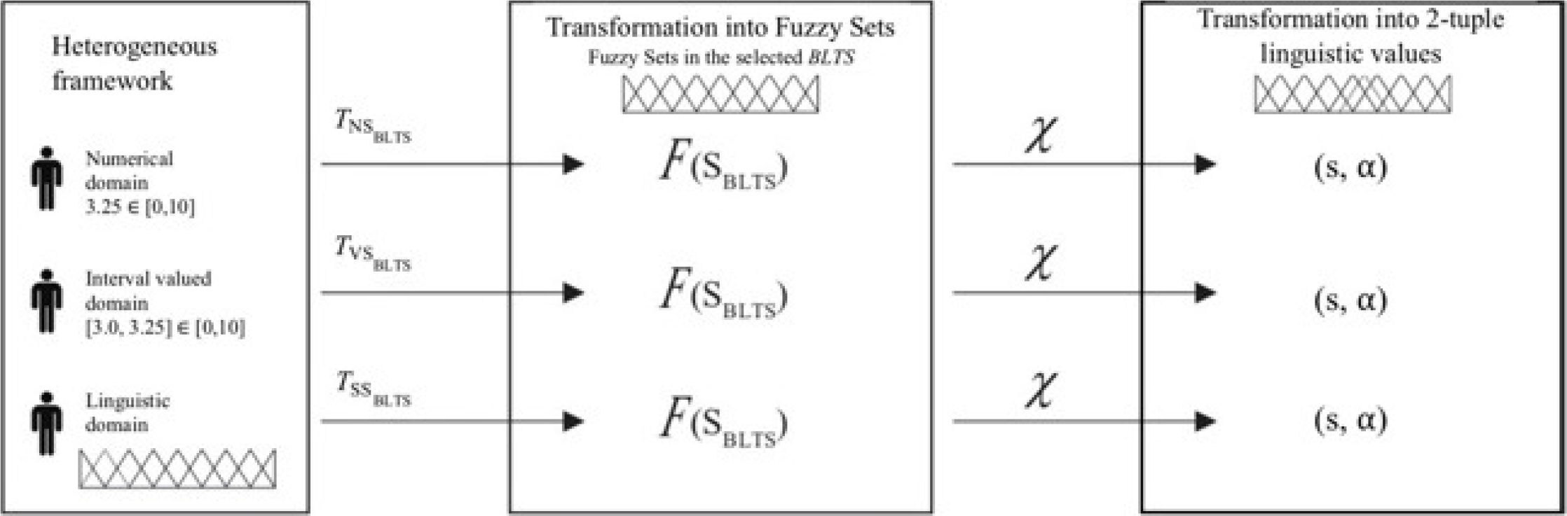
2.4 Transformation of Fuzzy Sets into Linguistic 2-tuple Values

Here, the fuzzy sets are converted into linguistic 2-tuples over the BLTS through the function χ:F(SBLTS)S×[0.5,0.5), which is stated as follows:

χ(λ0,λ1,,λh)=ΔS(i=0hiλii=0hλi)=(s,α)=s¯S¯BLTS, (21)

where S={S0,S1,,Sh} is the set of linguistic terms, and S¯={S0,S1,.,Sh} is the linked 2-tuple term set. The function ΔS is defined in section 2.2.2. After the transformations of heterogeneous information into 2-tuple linguistic values in the BLTS have been carried out, we can use the 2-tuple linguistic computation model [7] to compute linguistic results in S¯BLTS. This step uses 2-tuple linguistic aggregation operators [20, 22]. Based on the results presented in this section, we present a linguistic extension of the ELECTRE III method in the following section.

3 The Linguistic ELECTRE III Method

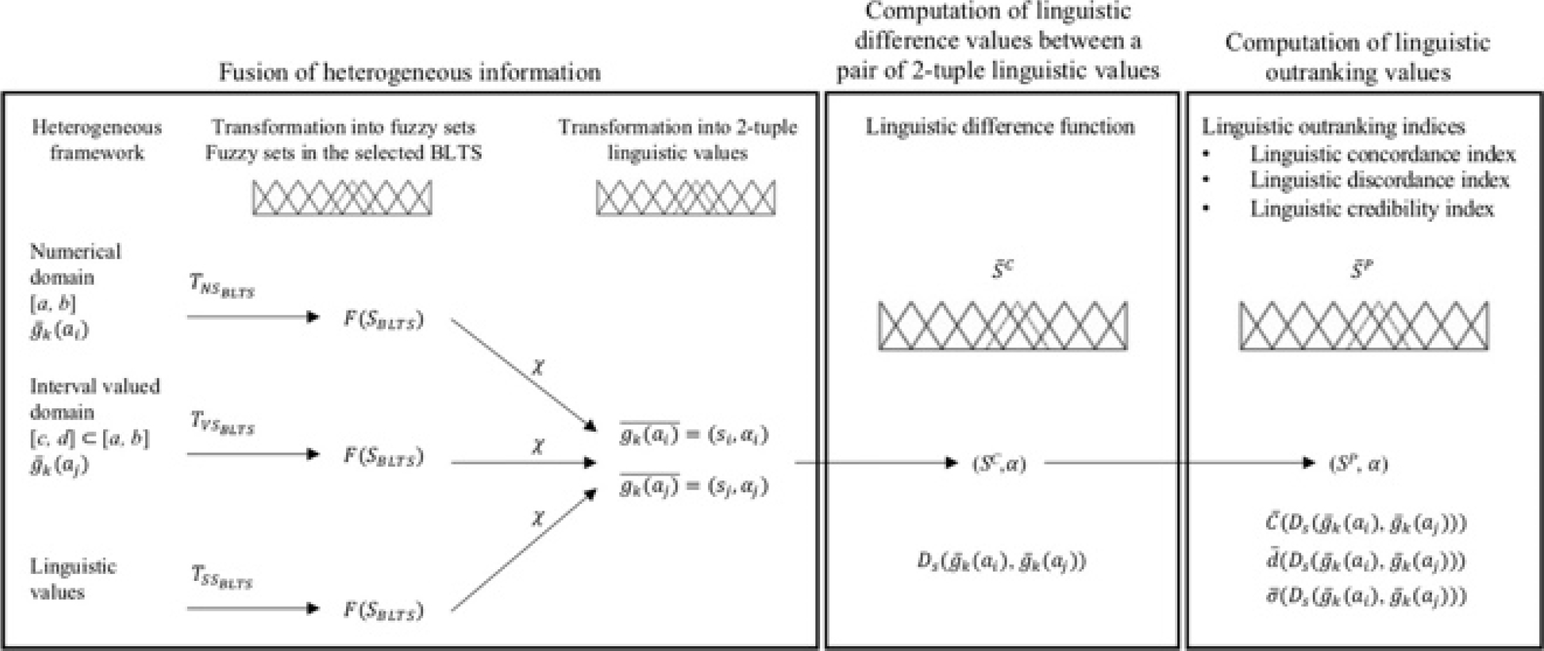
This section presents our proposal for the linguistic extension of the ELECTRE III model; to this end, a procedure is defined to model the partial and global concordance indices, the discordance indices by criterion, the thresholds of the criteria, and the credibility index linguistically so that they can accept 2-tuple linguistic values.

Consequently, the linguistic ELECTRE III method provides a more realistic operability of the qualitative criteria when solving multicriteria ranking problems.

Within this procedure, a linguistic difference function allows for the calculation of the linguistic difference for each pair of alternatives for each decision criterion. The linguistic output provided by the linguistic difference function serves as the linguistic input of the linguistic concordance and discordance indices for each criterion.

The output of the concordance and discordance indices are expressed in the same linguistic scale to preserve interpretability. Figure 2 schematically presents the process for modeling the linguistic outranking index in three phases.

Fig. 2 Process for modeling linguistic outranking indices 

3.1 Fusion of Heterogeneous Information

In a multicriteria ranking problem with a heterogeneous information environment, alternatives are evaluated using diverse expression domains based on the uncertainty and criteria type, as well as each DM's experience.

3.1.1 Transformation into Fuzzy Sets

The expression domains (numerical, interval, and linguistic) used in the heterogeneous framework are presented in this part of the first phase. The fusion approach handles these three types of information.

Previously, a unification domain SBLTS is defined as allowing the transforming of heterogeneous information by fuzzy sets into SBLTS, using the respective transformation functions of Eqs. 14, 16, and 19.

3.1.2 Transformation into 2-tuples Linguistic Values

Then, the process transforms the fuzzy sets into 2-tuple linguistic values in SBLTS using Eq. (21). Hence, the fused evaluation for each criterion gk concerning each alternative ai, is represented in a 2-tuple linguistic value g¯k(ai)=(si,αi)SBLTS.

3.2 The Linguistic Difference Function

This function is introduced to facilitate the computation of the linguistic concordance and discordance indices because the input values of the indices and thresholds must be linguistic values for a correct interpretation.

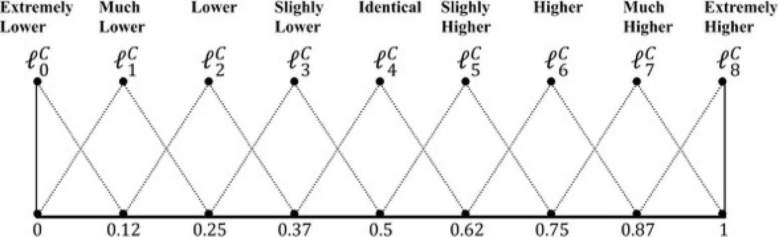
To compare two linguistic values, we need a comparison scale that can measure the linguistic difference between them. The scale's granularity will depend on the decision maker's knowledge, who needs to interpret the difference between the two alternatives using a bipolar scale [23]. This type of scale is convenient because it has a neutral point, which separates the positive differences from the negative ones [5].

In short, this function's linguistic output is the input of the linguistic concordance and discordance indices. The linguistic difference function is expressed in the linguistic scale, and the threshold parameters are stated accordingly. Consequently, a proper linguistic difference function between linguistic preference values is necessary for developing an extension of ELECTRE III dealing with fuzzy linguistic information.

Definition 3.1. Let SBLTS={s0,sh} and SC={l0C,,lhC} be the set of linguistic terms for preference values and the set of linguistic terms to express the linguistic difference value between two terms in SBLTS, respectively. Let (si,αi) and (sj,αj) be two 2-tuple linguistic values stated in SBLTS. The linguistic difference value between (si,αi) and (sj,αj) expressed in SC is calculated by:

DS:S¯BLTS×S¯BLTSS¯C, (22)

DS((si,αi),(sj,αj))=ΔSC(((ΔSBLTS1(sj,αj)ΔSBLTS1(si,αi))+h)2hh¯). (23)

The proposed linguistic difference function satisfies the following properties:

– The difference between the same value of SBLTS is the neutral point value of SC:

DS((si,αi),(si,αi))=neutralpoint{SC}=lh^/2C. (24)

– The difference between the minimum (maximum) and maximum (minimum) values of SBLTS must be the maximum (minimum) value of SC:

Ds((s0,0),(sh,0))=max{SC}=lhC,Ds((sh,0),(s0,0))=min{SC}=l0C. (25)

The proof of these properties is trivial. We propose the following syntax for SC:

SC={l0C:Extremely_Lower(EL),l1C:Much_Lower(ML),l2C:Lower(L),l3C:SlightlyLower(SL),l4C:Identical(I),l5C:SlightlyHigher(SH),l6C:Higher(H),l7C:Much_Higher(MH),l8C:Extremely_Higher(EH)}. (26)

Example 2. In this example, we perform the linguistic difference of the 2-tuple linguistic values (L,0.2) and (H,0,3) using the linguistic difference function (Definition 3.1). The set of linguistic terms for preference values is defined as follows:

SBLTS={s0:Very_low(VL),s1:Low(L),s2:Medium(M),s3:High(H),s4Very_high(VH)}. (27)

With the linguistic terms SC to describe the difference function defined above:

DS((L,0.2),(H,0.3))=ΔSC(((2.70.8)+4)(2)(4)8)=ΔSC(5.9)=(l5C,0.9)=(SH,0.9). (28)

3.3 Linguistic Concordance and Discordance Indices

The linguistic concordance and discordance indices defined in this section have 2-tuple linguistic values as input and output.

3.3.1 The Linguistic Concordance Index

The linguistic concordance value of (ai,aj)A×A for a criterion k is calculated by making use of a linguistic concordance index C¯k(ai,aj) through the linguistic difference function. The input value of the kth concordance index is a linguistic difference value of:

(ai,aj)A×ADS(g¯k(ai),g¯k(aj))S¯C, (29)

where gk:ASBLTS is the kth criteria function. The output value of the linguistic concordance function, i.e., the concordance value, is likewise represented by a value in a linguistic concordance scale S¯P.

SP={s0P,,shPP} represents a linguistic term set. The granularity of SP is chosen following the DM’s knowledge to make clear the concordance value of (ai,aj)A×A.

Here, (s0P,0) represents no concordance and (shPP,0) strict concordance.

The concordance index C¯k(ai,aj) varies from (s0P,0) to (shPP,0). If C¯k(ai,aj) is equal to (s0P,0), then ai is worse than aj.

The indifference and preference thresholds (ltqk,αqk)q and (ltpk,αpk)p respectively, both in S¯C, are used to construct a concordance index C¯k(ai,aj) for each criterion k, defined by:

Definition 3.2. The linguistic concordance index concerning a criterion gk, C¯k(ai,aj), that symbolizes the linguistic concordance value stated in 2-tuple linguistic values in SP={s0P,,shPP} of the linguistic difference value between aj over ai, regarding criterion k, D¯S(ai,aj)k=DS(g¯k(ai),g¯k(aj))SC is specified as:

C¯k(ai,aj):A×AS¯P, (30)

C¯k(ai,aj)={(S0P,0),ifD¯S(ai,aj)k>(ltpk,αpk)pΔSp(ΔSC1(ltpk,αpk)ph¯2[ΔSC1(D¯S(ai,ajΔSC1(ltpk,αpk)ph¯2(ΔSC1(ltqk,αqk)if(ltqk,αqk)q<D¯S(ai,aj)k(ltp(ShpP,0),ifD¯S(ai,aj)k(ltqk,αqk) (31)

With k=1,,n.

The concordance index C¯k(ai,aj) is a linguistic index measuring whether “ai is at least as good as aj” on criterion k.

3.3.2 The Linguistic Discordance Index

For each criterion gk a linguistic discordance index d¯k(ai,aj) can be defined. This index measures how much gk is more or less discordant with the affirmation “ai outranks aj.” This index considers a linguistic veto threshold (ltvk,αvk)v to calculate linguistic concordance.

It should be mentioned that any outranking of ai by aj by specified by the concordance index can be overruled if there is any criterion gk for which the alternative aj outperforms the alternative ai by at least a veto threshold, even if all the other criteria favor the outranking of ai(D¯S(ai,aj)k(ltvk,αvk)).

So, if ai is better than aj normally, there may be some criteria (possibly one) where ai is worse than aj. The index d¯k(ai,aj) displays this condition for that criterion. d¯k(ai,aj) varies from (shPP,0) to (shPP,0). (s0P,0) represents no discordance and (shPP,0) represents strict discordance. The linguistic discordance index is calculated according to the following definition:

Definition 3.3. The linguistic discordance index d¯k(ai,aj), for a criterion gk, that represents the linguistic discordance value expressed in 2-tuple linguistic values in SP={s0P,,shPP} of the linguistic difference value between aj over ai, regarding criterion k, D¯S(ai,aj)k=DS(g¯k(ai),g¯k(aj))S¯C is stated as:

d¯k(ai,aj):A×AS¯P, (32)

d¯k(ai,aj)={(S0P,0),ifDs(ai,aj)k(ltpk,αpk)pΔsp(Δsc1(D¯s(ai,aj)k)h¯2[Δsc1(ltpk,αpk)ph^2]Δsc1(ltvk,αvk)vh^2(Δsc1(ltpk,αpk)ph^2)hp),if(ltpk,αpk)p<D¯s(ai,aj)k<(ltvk,αvk)v(ShpP,0),ifD¯s(ai,aj)k(ltvk,αvk)v (33)

with k=1,,n.

3.4 The Linguistic Outranking Relation in the Linguistic ELECTRE III

The linguistic outranking relation OAσ¯ defined for each (ai,aj)A×A as a linguistic credibility index, σ¯(ai,aj)A×A, state broadly in what linguistic measure “ai outranks aj” employing both the linguistic concordance index C¯(ai,aj) and the linguistic discordance indices d¯k(ai,aj) for each criterion gk.

The linguistic credibility index is the comprehensive linguistic concordance index reduced by the linguistic discordance indices. In the nonappearance of such linguistic discordance criteria, σ¯(ai,aj)=C¯(ai,aj).

This linguistic credibility value is decreased in the occurrence of one or more linguistic discordant criteria gk when d¯k(ai,aj)>C¯(ai,aj). In correspondence with the veto effect σ¯(ai,aj)=(s0P,0) if exists a linguistic discordance index such that d¯k(ai,aj)=(shPP,0), does not matter what the weight of the criterion wk is. The linguistic credibility index σ¯(ai,aj) is defined as follows:

σ¯(ai,aj)={C¯(ai,aj),ifK¯(ai,aj)=ϕΔSP(ΔSP1(C¯(ai,aj))kK¯(ai,aj)ΔSP1(shPP,0)ΔSP1(d¯k(ai,aj))ΔSP1(shPP,0)ΔSP1(C¯(ai,aj)))ifK¯(ai,aj)ϕ, (34)

where:

K¯(ai,aj)={gkG|d¯k(ai,aj)>C¯(ai,aj)}. (35)

The formula for determining the linguistic value of σ¯(ai,aj) over the linguistic interval ((s0P,0),(shPP,0)) is non-compensatory, i.e., an alternative’s notable poor performances in some criteria cannot be compensated for even with very high performance in other criteria. The aggregated performance exposes this fact. This completes the first phase of the linguistic ELECTRE III method.

3.5 The Ranking Algorithm in the Linguistic Extension of ELECTRE III

The second phase of the linguistic ELECTRE method is to exploit the linguistic outranking relation OAσ¯ to get a partial preorder of the alternatives. This final partial preorder is obtained because of the “intersection” of two complete preorders resulting from the descending and ascending distillations [24].

In the descending distillation, the procedure ranks the alternatives from the best to the worst; on the contrary, in the ascending distillation, the process ranks the alternatives from the worst to the best.

In the following, we modify the distillation procedure of ELECTRE III. In the linguistic ELECTRE III distillation procedure, we state a set of linguistic credibility cutting levels (stc,αc)(r) in SP={s0P,,shPP}. Given a linguistic cutoff level symbolized by (stc,ac)(r), both distillations relate to the following linguistic crisp outranking relation:

aiOA(stc,αc)(r)aj (36)

{σ¯(ai,aj)(stc,αc)(r)σ¯(ai,aj)>ΔSP(ΔSP1(σ¯(aj,ai))+z(σ¯(ai,aj))),

where z(λ¯)=α(ΔSP1(λ¯))hP+β is a linguistic distillation threshold and α and β are two distillation coefficients. (stc,αc)(r) is also a linguistic preference parameter, which fixes the minimum degree of credibility considered obligatory by the DM to support the statement “ai outranks aj”. From the linguistic crisp outranking relation, for each alternative ai, its (stc,αc)(r)-qualification is:

qA(stc,αc)(r)(ai)=pA(stc,αc)(r)(ai)fA(stc,αc)(r)(ai), (37)

where pA(stc,αc)(r)(ai)=|{ajA:aiOA(stc,αc)(r)aj}| is the (stc,αc)(r)-power of ai; it is the number of alternatives that are outranked by ai, and fA(stc,αc)(r)(ai)=|{ajA:ajOA(stc,αc)(r)ai}| is the (stc,αc)(r)-weakness of ai; it is the number of alternatives outranking ai.

In the rest of this section, we explain the descending and ascending distillation algorithms in detail as follows: Let (stc,αc)(1) be the first fixed linguistic cutoff level and qA(stc,αc)(1)(ai) be the

qualification of alternative ai. Then, choose in A the best ones resulting a subset of alternatives from A that has the maximum qualification (descending selection, D1) or the worst alternatives resulting thus a subset of alternatives from A, which has the minimum qualification (ascending selection, D1:

D1={aiA|qA(stc,αc)(1)(ai)=qA=maxxAqA(stc,αc)(1)(x)}, (38)

D1={aiA|qA(stc,αc)(1)(ai)=qA=minqA(stc,αc)(1)(x)xA}. (39)

Consequently, at the end of the k steps of the first distillation, the first subset of A is obtained, representing the first (last) class of one of the two final preorders. Let C1=Dk symbolize the first class of the descending selection, and C1=Dk indicate the last class of the ascending selection.

Let A1=A\C1, or A1=A\C1 represent the remaining subset of the alternatives from A to rank after the first distillation. In A1 and A1 The alternatives’ qualification is computed again for choosing one or various alternatives. This process is reiterated until all the alternatives are ranked.

The distillation process is condensed in the following way:

  1. Set n=0, put or A0=A (descending), or A0=A (ascending).

  2. Set: (stc,αc)(0)=maxai,ajAnaiajσ¯(ai,aj)or(stc,αc)(0)=maxai,ajAnaiajσ¯(ai,aj).

  3. Put k=0,D0=An (descending) or D0=An (ascending).

  4. Choose the maximum value from the linguistic credibility scores that are less than (stc,αc)(k)z((stc,αc)(k)).

  5. (stc,αc)(k+1)=max{σ¯(ai,aj)+z((stc,αc)(k))<(stc,αc)(k)}ai,ajDkσ¯(ai,aj).

  6. ifai,ajDk,σ¯(ai,aj)+z((stc,αc)(k))>(stc,αc)(k),put(stc,αc)(k+1)=(s0,0).

  7. Calculate the (stcαc)(k+1)-qualifications (qA(stc,αc)(k)(ai))aiDk.

  8. Obtain the maximum or minimum (stc,αc)(k+1)-qualification score: qDk=maxqDk(stc,αc)(k)(x)xDk (descending) or qDk=minqDk(stc,αc)(k)(x)xDk (ascending).

  9. Construct Dk+1={aiDk|qDk(stc,αc)(k+1)(ai)=qDk} (descending) or Dk+1={aiDk|qDk(stc,αc)(k+1)(ai)=qDk} (ascending).

  10. If |Dk+1|=1or|Dk+1|=1or(stc,αc)(k+1)=(s0,0) you proceed to step (9).

  11. else, do k=k+1, Dk=Dk (descending) or Dk=Dk (ascending) and go to step (4).

  12. Cn+1=Dk+1 is the set of alternatives carried through the (n+1)th downward distillation, termed the (n+1)th distillate of the downward procedure. Cn+1=Dk+1 is the set of alternatives taken through the (n+1)th upward distillation, termed the (n+1)th distillate of the upward procedure.

  13. Put An+1=An\Cn+1 (descending) or An+1=An\Cn+1 (ascending).

  14. If An+1ϕ,orAn+1ϕ then n=n+1, and proceed to Step (2).

  15. Otherwise, end of the distillation.

During the same distillations, when advancing from step k to step k+1, the linguistic cutoff level (stc,αc)(k) is replaced by (stc,αc)(k+1)<(stc,αc)(k) as follows (Dk is the remaining set of alternatives to rank):

(stc,αc)(k+1)=max{σ¯(ai,aj)+z((stc,αc)(k))<(stc,αc)(k)}ai,ajDk,σ¯(ai,aj) (40)

where z((stc,αc)(k))=ΔSP(α(ΔSP1((stc,αc)(k)))hP+β).

The analyst can fix one value for the distillation coefficients α and β before the computations. The standard values recommended in the literature are α=0.15 and β=0.30.

We obtain two complete preorders at the end of the distillation procedure. In each preorder, the alternatives are regrouped in a partition of equivalence classes, forming a ranking from the best to the worst alternatives.

Each class includes at least one alternative. A partial preorder of the alternatives is constructed utilizing the intersection of both preorders, which specifies the comparisons between alternatives and emphasizes the possible incomparabilities as follows:

  • – Alternative ai is preferred to the alternative aj if ai belongs to a class not worse than alternative aj in both preorders and a better class for at least one of the two preorders.

  • – Alternative ai is indifferent to alternative aj if ai and aj belong to the same class in the two preorders.

  • – Alternatives ai and aj are incomparable if ai belongs to a class better than aj in one preorder and worse in the other or vice versa.

To illustrate the proposed method, we present in the following section a step-by-step example of the linguistic ELECTRE III method for ranking a set of alternatives.

4 An Illustrative Example

We will use a case study from [25] to demonstrate the proposed approach. This case study is an Environmental Impact Significance Assessment problem in which heterogenous data (qualitative and quantitative judgments) obtained from a DM are used to determine the environmental impacts that a set of projects or industrial activities can have on a petrol station's usual operations.

This case study aims to evaluate seven ecological effects that can occur between the interactions of four industrial activities and four environmental factors in a petrol station. The evaluation seeks to rank the identified impacts from the most to the least significant. Each step of the linguistic extension of the ELECTRE III method is explained below.

Step 1. Formulation of the multicriteria ranking problem. Given a set of activities from a petrol station A = {a1: The operation of petrol pumps, a2: the operation of the car wash, a3: the transport of fuel and materials, and a4: the filling of fuel tanks} and four possible environmental factors F = {f1: Daily sound comfort, f2: hydrocarbons in the air, f3: public health and civic safety, and f4: energy infrastructures} a set of seven possible environmental impacts that are triggered from the interaction between A and F, was identified EI = {(a1,f2),(a1,f3),(a2,f1),(a2,f4),(a3,f1),(a3,f4),(a4,f1)}.

For convenience, we define EI = {ei1,ei2,ei3,ei4,ei5,ei6,ei7}. For the assessment of the elements in EI, a DM, which has specific knowledge is public health, expressed his preferences on EI using diverse expression domains: Numerical(N), Interval-valued(I), or Linguistic (L) over a set of 10 criteria defined in Table 1. Note that the preference direction for all criteria is to maximize.

Table 1 Criteria set description 

Name Description Expression Domain
g1 Intensity How the action impacts the factor Linguistic: L
g2 Extension The range within which the action affects the site Linguistic: L
g3 Moment The duration from the action’s onset to the time the factor begins to be affected Numerical: N
g4 Persistence The estimated duration of the action’s effect Valor Interval-valued: I
g5 Reversibility The potential for the factor to be naturally restored to its original state after being affected Numerical: N
g6 Synergy The strengthening of straightforward impacts Linguistic: L
g7 Accumulation The gradual escalation in the expression of the effect Linguistic: L
g8 Effect How the action’s impact on an environmental factor becomes apparent Linguistic: L
g9 Recoverability The potential for the factor to be restored with the help of human action Linguistic: L
g10 Periodicity The consistency in which the impact on the environmental factor is observed Linguistic: L

The DM uses a linguistic domain with five linguistic terms denoted by S5 to express his/her preferences. Each linguistic term set is symmetrically and uniformly distributed, and its syntax is defined in the following form:

S5={S0:VeryLow(VL),S1:Low(L),S2:Medium(M)S3:High(H),S4:VeryHigh(VH). (41)

Step 2. Collecting the heterogeneous information: The DM assessed each criterion for each impact in EI using a heterogeneous framework. The expression domain used for each criterion was according to its nature; for criteria g1, g2, g6, g7, g8, g9, and g10 were used the linguistic terms in S5; for criteria g3 and g5 were used a scale based on real numbers; meanwhile, for criterion g4 was used an interval scale. The assessment made by the DM is presented in Table 2.

Table 2 Assessment for each criterion on each EI using a heterogeneous framework 

g1 g2 g3 g4 g5 g6 g7 g8 g9 g10
ei1 L L 0,00 [0,0.2] 1,00 L L L H VL
ei2 H VL 0,00 [0,0.2] 1,00 M M M VH VL
ei3 H L 0,00 [0.4,0.6] 10,00 M L VH L M
ei4 M VL 0,10 [0,0.2] 2,00 L VL VL M H
ei5 H L 0,10 [0,0.05] 10,00 M M VH L M
ei6 VH L 0,00 [0.8,1.0] 10,00 M M VH L H
ei7 VL L 1,50 [0.8,1.0] 10,00 VL L VL L VH

Step 3. Fusion of the heterogeneous information: The chosen linguistic domain to fuse the information is S5. The integrated information given by the DM is shown in Table 3.

Table 3 Fused information supplied by the DM 

g1 g2 g3 g4 g5 g6 g7 g8 g9 g10
ei1 (L,0) (L,0) (VH,0) (VL,0.44) (VL,0.4) (L,0) (L,0) (L,0) (H,0) (VL,0)
ei2 (H,0) (VL,0) (VH,0) (VL,0.44) (VL,0.4) (M,0) (M,0) (M,0) (VH,0) (VL,0)
ei3 (H,0) (L,0) (VH,0) (M,0) (VH,0) (M,0) (L,0) (VH,0) (L,0) (M,0)
ei4 (M,0) (VL,0) (VH,-0.04) (VL,0.44) (L,-0.2) (L,0) (VL,0) (VL,0) (M,0) (H,0)
ei5 (H,0) (L,0) (VH,-0.04) (VL,0.17) (VH,0) (M,0) (M,0) (VH,0) (L,0) (M,0)
ei6 (VH,0) (L,0) (VH,0) (VH,-0.44) (VH,0) (M,0) (M,0) (VH,0) (L,0) (H,0)
ei7 (VL,0) (L,0) (H,0.4) (VH,-0.44) (VH,0) (VL,0) (L,0) (VL,0) (L,0) (VH,0)

Step 4. Computing linguistic difference values between unified assessments: The linguistic difference value between a pair of 2-tuple linguistic values is stated in the linguistic comparison scale SC presented in Figure 3. Linguistic difference values are calculated by Eq. (23).

Fig. 3 Linguistic comparison scale SC 

Step 5. Computing linguistic concordance values: Linguistic concordance index concerning a criterion gk, Ck(eii,eij).

Calculations to get individual linguistic concordance values. Initially, the linguistic preference scale SP is chosen. After that, for each criterion gk, its linguistic concordance function is performed (Eq. (31)) and its indifference and preference threshold parameters are defined in 2-tuple linguistic values in SC.

Each linguistic concordance value for each alternative eii, with regards to alternative eij, over a criterion gk, is calculated using the linguistic outranking function (Eq. 31).

The calculation of the linguistic outranking value for each criterion is given in a linguistic preference scale SP={S0P,,SkP} with nine linguistic terms. The inter-criteria parameters of gk, k=1,2,,10 are presented in Table 4, which are described in SC.

Table 4 Indifference q preference p and veto v values 

Criterion ((ItqkC,αqk)q) ((ItpkC,αpk)p) ((ItckC,αvk)v)
g1 (I5C,0)q (I6C,0)p (I7C,0)v
g2 (I5C,0)q (I6C,0)p (I7C,0)v
g3 (I5C,0)q (I6C,0)p
g4 (I5C,0)q (I6C,0)p
g5 (I5C,0)q (I6C,0)p
g6 (I5C,0)q (I6C,0)p
g7 (I5C,0)q (I6C,0)p
g8 (I5C,0)q (I6C,0)p
g9 (I5C,0)q (I6C,0)p
g10 (I5C,0)q (I6C,0)p

Example 3. Calculation of C¯1(ei1,ei6). According to the descriptive example, the computations of the linguistic concordance indices (Definition 3.2) can be made in the following form: From Table 3, g¯1(ei1)=(L,0) and g¯1(ei6)=(VH,0), then:

DS(ei1,ei6)1=DS(g¯1(ei1),g¯1(ei6))1=DS((L,0),(VH,0))1=ΔSC((ΔSBLTS1(VH,0)ΔSBLTS1(L,0))+82x8×8)=ΔSC((41)+82x8×8)=ΔSC(5.5)=(I5C,0.5). (42)

Based on Eq. (31), since:

(I5C,0)qDS(ei1,ei6)1=(I5C,0.5)(I6C,0)p. (43)

Then from interpolation, we calculate:

C¯1(ei1,ei6)=((I6C,0)p82((I5C,0.5)82)(I6C,0)p82((I5C,0)q82))×8=(I4C,0). (44)

In this way, it is possible to get the linguistic concordance indices C¯k(eii,eij) on a criterion gk for all pairs of alternatives (eii,eij), and, finally, display the linguistic concordance matrices for each criterion.

For example, on the criterion g1 the linguistic concordance matrix is expressed in Table 5. The comprehensive linguistic concordance index C¯(eii,eij).

Table 5 Concordance indices on the criterion g1 

ei1 ei2 ei3 ei4 ei5 ei6 ei7
ei1 (S8P,0) (S8P,0) (S8P,0) (S8P,0) (S8P,0) (S4P,0) (S8P,0)
ei2 (S8P,0) (S8P,0) (S8P,0) (S8P,0) (S8P,0) (S8P,0) (S8P,0)
ei3 (S8P,0) (S8P,0) (S8P,0) (S8P,0) (S8P,0) (S8P,0) (S8P,0)
ei4 (S8P,0) (S8P,0) (S8P,0) (S8P,0) (S8P,0) (S8P,0) (S8P,0)
ei5 (S8P,0) (S8P,0) (S8P,0) (S8P,0) (S8P,0) (S8P,0) (S8P,0)
ei6 (S8P,0) (S8P,0) (S8P,0) (S8P,0) (S8P,0) (S8P,0) (S8P,0)
ei7 (S8P,0) (S4P,0) (S4P,0) (S8P,0) (S4P,0) (S4P,0) (S8P,0)

The comprehensive linguistic concordance index C¯(eii,eij) is computed using the weight vector:

W=(0.36,0.24,0.08,0.04,0.04,0.04,0.04,0.04,0.08,0.04)

for the family of criteria. The value of C¯(ei1,ei6) is computed as follows:

C¯(ei1,ei6)=ΔSP(0.36(ΔSP1(C¯1(ei1,ei6))+0.24(ΔSP1(C¯2(ei1,ei6))+0.08(ΔSP1(C¯3(ei1,ei6))+0.04(ΔSP1(C¯4(ei1,ei6))+0.04(ΔSP1(C¯5(ei1,ei6))+0.04(ΔSP1(C¯6(ei1,ei6))+0.04(ΔSP1(C¯7(ei1,ei6))+0.04(ΔSP1(C¯8(ei1,ei6))+0.08(ΔSP1(C¯9(ei1,ei6))+0.04(ΔSP1(C¯10(ei1,ei6)))=(S5P,0.8048). (45)

Proceeding in the same way, for all pairs of environmental impacts (ei1,eij) representing the illustrative example, the comprehensive linguistic concordance matrix is obtained (Table 6).

Table 6 Comprehensive linguistic concordance matrix C¯(eii,eij) 

C¯(eii,eij) ei1 ei2 ei3 ei4 ei5 ei6 ei7
ei1 (S8P,0) (S8P,0) (S7P,0.584) (S7P,0.84) (S7P,0.584) (S5P,0.8048) (S7P,0.2448)
ei2 (S8P,0) (S8P,0) (S7P,0.744) (S7P,0.84) (S7P,0.744) (S7P,0.4048) (S7P,0.2448)
ei3 (S8P,0) (S7P,0.68) (S8P,0) (S8P,0) (S8P,0) (S8P,0) (S8P,0)
ei4 (S8P,0) (S8P,0) (S7P,0.488) (S8P,0) (S7P,0.488) (S7P,0.3088) (S7P,0.6288)
ei5 (S8P,0) (S7P,0.68) (S8P,0) (S8P,0) (S8P,0) (S7P,0.7776) (S7P,0.7776)
ei6 (S8P,0) (S7P,0.68) (S8P,0) (S8P,0) (S8P,0) (S8P,0) (S8P,0)
ei7 (S8P,0) (S6P,0.24) (S6P,0.24) (S8P,0) (S6P,0.24) (S4P,0.8) (S8P,0)

Step 6. Computing linguistic discordance values d have been defined on criteria d¯k(eii,eij). The linguistic veto thresholds g1 and g2. These criteria can give a linguistic discordance index that is not null.

Example 4. Calculation of d¯1(ei1,ei6). The computations of the linguistic discordance indices (Definition3.3) can be made as follows: from Table 3 g¯1(ei1)=(L,0) and g¯1(ei6)=(VH,0), from example 2 DS(ei1,ei6)1=(I5C,0.5).

Since DS(ei1,ei6)1=(I5C,0.5)(I6C,0)P then from Eq. 42 d¯1(ei1,ei6)=(S0P,0).

In the same way, with this computation process, it is possible to obtain the linguistic discordance indices d¯k(eii,eij) on the criterion gk for all pairs of environmental impacts (eii,eij) and display the linguistic discordance matrices for each criterion where it is defined a linguistic veto threshold. For instance, on the criterion g1, the computed discordance matrix is defined in Table 7.

Table 7 Linguistic discordance matrix on a criterion g1 

ei1 ei2 ei3 ei4 ei5 ei6 ei7
ei1 (S0P,0) (S0P,0) (S0P,0) (S0P,0) (S0P,0) (S0P,0) (S0P,0)
ei2 (S0P,0) (S0P,0) (S0P,0) (S0P,0) (S0P,0) (S0P,0) (S0P,0)
ei3 (S0P,0) (S0P,0) (S0P,0) (S0P,0) (S0P,0) (S0P,0) (S0P,0)
ei4 (S0P,0) (S0P,0) (S0P,0) (S0P,0) (S0P,0) (S0P,0) (S0P,0)
ei5 (S0P,0) (S0P,0) (S0P,0) (S0P,0) (S0P,0) (S0P,0) (S0P,0)
ei6 (S0P,0) (S0P,0) (S0P,0) (S0P,0) (S0P,0) (S0P,0) (S0P,0)
ei7 (S0P,0) (S0P,0) (S0P,0) (S0P,0) (S0P,0) (S0P,0) (S0P,0)

Step 7. Computing the linguistic outranking relation. Based on the comprehensive linguistic concordance matrix and the partial linguistic discordance matrices, the value of σ¯(ei1,ei6) is computed as follows:

Since K¯(ei1,ei6)=0 and k, d¯k(ei1,ei6)<C¯(ei1,ei6), then, from Eq. (21), σ¯(ei1,ei6)=C¯(ei1,ei6)=(S5P,0.8048).

For all pairs of alternatives representing the illustrative example, the linguistic credibility matrix or linguistic outranking matrix is obtained (see Table 8).

Table 8 Linguistic credibility matrix in the linguistic extension of the ELECTRE III 

C¯(eii,eij) ei1 ei2 ei3 ei4 ei5 ei6 ei7
ei1 (S8P,0) (S8P,0) (S7P,0.584) (S7P,0.84) (S7P,0.584) (S5P,0.8048) (S7P,0.2448)
ei2 (S8P,0) (S8P,0) (S7P,0.744) (S7P,0.84) (S7P,0.744) (S7P,0.4048) (S7P,0.2448)
ei3 (S8P,0) (S7P,0.68) (S8P,0) (S8P,0) (S8P,0) (S8P,0) (S8P,0)
ei4 (S8P,0) (S8P,0) (S7P,0.488) (S8P,0) (S7P,0.488) (S7P,0.3088) (S7P,0.6288)
ei5 (S8P,0) (S7P,0.68) (S8P,0) (S8P,0) (S8P,0) (S7P,0.7776) (S7P,0.7776)
ei6 (S8P,0) (S7P,0.68) (S8P,0) (S8P,0) (S8P,0) (S8P,0) (S8P,0)
ei7 (S8P,0) (S6P,0.24) (S6P,0.24) (S8P,0) (S6P,0.24) (S4P,0.8) (S8P,0)

Step 8. Ranking of alternatives from the linguistic outranking relation OAσ . The ranking algorithm can be applied according to the linguistic credibility matrix obtained by the linguistic ELECTRE III (Table 6).

For illustration purposes, we describe the procedure followed to perform the first four descending distillations as follows:

Let:

EI0=EI={ei1,ei2,ei3,ei4,ei5,ei6,ei7},z(λ¯)=ΔSp(α(ΔSp1(λ¯))hp+β). (46)

With α=0.15,β=0.30.

Distillation 1.

Step 1: Let n=0, EI0={ei1,ei2,ei3,ei4,ei5,ei6,ei7}, k=0 then (Stc,αc)(0)=maxa,bEI0ab(a,b)=(S8P,0), and D0=EI0, hence (Stc,αc)(1)=max{σ(a,b)+z((Stc,αc)(0))<(Stc,αc)(0)}a,bD0σ¯(a,b)=(S7P,0.84). Given this linguistic cutoff, we can create a linguistic crisp outranking relation using Eq. (36). Table 9 shows the resulting crisp outranking relation. From the crisp outranking relation, we calculate the (Stc,αc)(1)-qualifications (qA(Stc,αc)(0)(a))aD0 Table 10 shows the calculated power, weakness, and qualification.

Table 9 Crisp outranking relation 

eiiOeij ei1 ei2 ei3
ei1 0 0 0
ei2 0 0 0
ei3 1 0 0
ei4 1 1 0
ei5 1 0 0
ei6 1 0 0
ei7 1 0 0

Table 10 Power, weakness, and qualification scores 

eiiOeij ei1 ei2 ei3 ei4 ei5 ei6 ei7
pD0(stc,αc)(0) - power 0 0 3 2 2 4 2
fD(stc,αc)(0) - weakness 5 1 0 4 1 0 2
qD0(stc,αc)(0) - qualification 5 1 3 2 1 4 0

The maximum (Stc,αc)(k+1)-qualification score is qDk=maxxDkqDk(Stc,αc)(k)(x)=4, then: Dk+1={aDk|qDk(stc,αc)(k+1)(a)=qDk}, D1={ei6}. Because |D1|=1 then C1=D1={ei} and the first distillation is completed. For the subsequent distillation, put EI1=EI0\C1={ei1,ei2,ei3,ei4,ei5,ei6,ei7}\{ei6}={ei1,ei2,ei3,ei4,ei5,ei7} and do do n=n+1=1.

Distillation 2.

Step 1: Let k=0, D0=EI1={ei1,ei2,ei3,ei4,ei5,ei7}, then (Stc,αc)(0)=maxa,bEI0abσ¯(a,b)=(S8P,0), and (Stc,αc)(1)=max{σ(a,b)+z((Stc,αc)(0))<(Stc,αc)(0)}a,bD0σ¯(a,b)=(S7P,0.84).

From this linguistic cutoff, we create the linguistic crisp outranking relation shown in Table 11. Then we calculate the (Stc,αc)(1)-qualifications (qA(Stc,αc)(0)(a))aD0. Table 12 shows the calculated power, weakness, and qualification for D0 in step one of distillation 2. The maximum (Stc,αc)(k+1)-qualification score is qDk=maxxDkqDk(Stc,αc)(k)(x)=3, then Dk+1={aDk|qDk(stc,αc)(k+1)(a)=qDk}, D1={ei3}.

Table 11 Crisp outranking relation for iteration 1 in Distillation 2 

eiiOeij ei1 ei2 ei3 ei4 ei5 ei7
ei1 0 0 0 0 0 0
ei2 0 0 0 0 0 0
ei3 1 0 0 1 0 1
ei4 1 1 0 0 0 0
ei5 1 0 0 1 0 0
ei7 1 0 0 1 0 0

Table 12 Power, weakness, and qualification scores for iteration 1 in Distillation 2 

eiiOeij ei1 ei2 ei3 ei4 ei5 ei7
pD0(stc,αc)(0) - power 0 0 3 2 2 2
fD(stc,αc)(0) - weakness 4 1 0 3 0 2
qD0(stc,αc)(0) - qualification 4 1 3 1 2 0

Because |D1|=1 then C2=D1={ei3} and the first distillation is completed. For the subsequent distillation, put EI2=EI1\C2={ei1,ei2,ei3,ei4,ei5,ei7}\{ei3}={ei1,ei2,ei4,ei5,ei7} and do do n=n+1=2.

Distillation 3.

Iteration 1: Let k=0, D0=EI2={ei1,ei2,ei4,ei5,ei7}, then (Stc,αc)(0)=maxa,bEI2abσ¯(a,b)=(S8P,0), and (Stc,αc)(1)=max{σ(a,b)+z((Stc,αc)(0))<(Stc,αc)(0)}a,bD0σ¯(a,b)=(S7P,0.84).

From this linguistic cutoff, we create the linguistic crisp outranking relation shown in Table 13. Then we calculate the (Stc,αc)(1)-qualifications (qA(Stc,αc)(0)(a))aD0. Table 14 shows the calculated power, weakness, and qualification for D0 in Iteration one of distillation 3. The maximum (Stc,αc)(k+1)-qualification score is qDk=maxxDkqDk(Stc,αc)(k)(x)=2, then Dk+1={aDk|qDk(stc,αc)(k+1)(a)=qDk}, D1={ei5,ei7}. Because |D1|>1 we proceed with another iteration in distillation three.

Table 13 Crisp outranking relation for iteration 1 in Distillation 3 

eiiOeij ei1 ei2 ei4 ei5 ei7
ei1 0 0 0 0 0
ei2 0 0 0 0 0
ei4 1 1 0 0 0
ei5 1 0 1 0 0
ei7 1 0 1 0 0

Table 14 Power, weakness, and qualification scores for iteration 1 in Distillation 3 

eiiOeij ei1 ei2 ei4 ei5 ei7
pD0(stc,αc)(0) - power 0 0 2 2 2
fD(stc,αc)(0) - weakness 3 1 2 0 0
qD0(stc,αc)(0) - qualification 3 1 0 2 2

Iteration 2: Let k=1, and (Stc,αc)(2)=max{σ(a,b)+z((Stc,αc)(1))<(Stc,αc)(1)}a,bD1σ¯(a,b)=(S6P,0.24).

From this linguistic cutoff, we create the linguistic crisp outranking relation shown in Table 15. Then we calculate the (Stc,αc)(2)-qualifications (qA(Stc,αc)(1)(a))aD1. Table 16 shows the calculated power, weakness, and qualification for D1 in Iteration 2 of distillation 3.

Table 15 Crisp outranking relation for iteration 2 in distillation 3 

eiiOeij ei5 ei7
ei5 0 1
ei7 0 0

Table 16 Power, weakness, and qualification scores for iteration 2 in distillation 3 

eiiOeij ei5 ei7
pD0(stc,αc)(0)-power 1 0
fD(stc,αc)(0)-weakness 0 1
qD0(stc,αc)(0)-qualification 1 -1

The maximum (Stc,αc)(k+1)-qualification score is qDk=maxxDkqDk(Stc,αc)(k)(x)=1, then

Dk+1={aDk|qDk(stc,αc)(k+1)(a)=qDk}, (47)

D1={ei5}.

Because |D1|=1 then C3=D1={ei5} and the first distillation is completed. For the subsequent distillation, put EI3=EI2\C3={ei1,ei2,ei4,ei5,ei7}\{ei5}={ei1,ei2,ei4,ei7} and do n=n+1=3.

Distillation 4

Iteration 1: Let k=0, D0=EI3={ei1,ei2,ei4,ei7}, then (Stc,αc)(0)=maxa,bEI3abσ¯(a,b)=(S8P,0), and (Stc,αc)(2)=max{σ(a,b)+z((Stc,αc)(1))<(Stc,αc)(1)}a,bD1σ¯(a,b)=(S7P,0.84). From this linguistic cutoff, we create the linguistic crisp outranking relation shown in Table 17. Then we calculate the (Stc,αc)(1)-qualifications (qA(Stc,αc)(0)(a))aD0. Table 18 shows the calculated power, weakness, and qualification for D0 in step one of distillation 4. The maximum (Stc,αc)(k+1)-qualification score is qDk=maxxDkqDk(Stc,αc)(k)(x)=1, then Dk+1={aDk|qDk(stc,αc)(k+1)(a)=qDk}, D1={ei7}. Because |D1|=1 then C4=D1={ei7} and the third distillation is completed. For the subsequent distillation, put EI4=EI3\C4={ei1,ei2,ei4,ei7}\{ei7}={ei1,ei2,ei4,} and do do n=n+1=4.

Table 17 Crisp outranking relation for iteration 1 in distillation 4 

eiiOeij ei1 ei2 ei4 ei7
ei1 0 0 0 0
ei2 0 0 0 0
ei4 1 1 0 0
ei7 1 0 1 0

Table 18 Power, weakness, and qualification scores for iteration 1 in distillation 4 

eiiOeij ei1 ei2 ei4 ei7
pD0(stc,αc)(0) - power 0 0 2 2
fD(stc,αc)(0) - weakness 2 1 1 0
qD0(stc,αc)(0) - qualification 2 1 1 2

The remaining steps for the next descending distillations and the ascending distillation steps are processed in the same way. After completing the descending and ascending distillations, we got two complete preorders whose intersection creates the final ranking of the alternatives.

Figure 4 depicts the two preorders (descending and ascending distillations) calculated with the distillation procedure. In the descending preorder (Fig 4. a), there is an equivalence class in the first rank with the environmental impacts ei1, ei2, ei4, ei7, followed by EI ei5 in the second rank, and at the last rank, there is an equivalence class with the environmental impacts ei3 and ei6. Meanwhile, the ascending distillation (Fig 4. b) is more granulated with ei1 in the first rank, followed by ei4ei7ei5ei2, and at the last rank are ei3 and ei6.

Fig. 4 Graphical representation of the preorders 

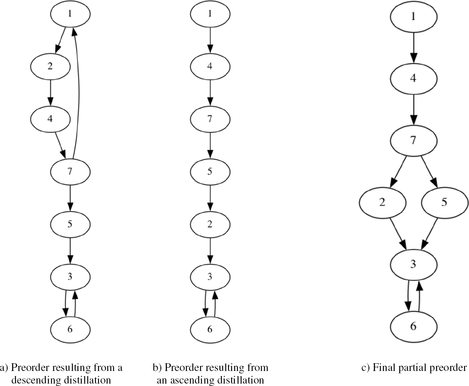
Figure 4. c depicts the final preorder resulting from the intersection of the two preorders.

The final partial preorder follows a decreasing order of preferences, meaning that environmental impacts at the top are more significant than those at the bottom.

Hence, the final rank suggests that the ei1 is the most significant environmental impact that is the interaction between action a1 and factor f2; in the second position is ei4, that is the interaction between action a2 and factor f4; in the third position is ei7 that is the interaction between action a4 and factor f1; in the fourth position are ei2 and ei5 that are the interactions between a1 and factor f3, and a3 and factor f1 respectively; it should be noted that although ei2 and ei5 are in the same ranking, they are incomparable. Thus, more analysis should be made for these two actions; finally, in the last rank, there is an equivalence class with ei3 and ei6 that suggests that both are indifferent to each other.

5 Conclusions

This paper aimed to develop a linguistic extension of the ELECTRE III method that allows solving instances of the multicriteria ranking problem with input data defined in heterogeneous contexts.

The new proposal fuses the heterogeneous information into 2-tuple linguistic values, allowing the DM to provide their preferences using diverse expression domains, such as numerical domain, interval-valued domain, and linguistic domain, according to the nature and uncertainty of the decision criteria, and their level of knowledge and experience.

Consequently, the new method is appropriate to integrate quantitative and qualitative criteria and uncertain information into the elements of the multicriteria model. In the modeling process of the ELECTRE III linguistic method, concordance, discordance, and credibility indices are proposed to consider linguistic inputs and outputs. Also, a linguistic difference function is stated to compute the linguistic difference between a pair of 2-tuple linguistic values. The output of the linguistic difference function is the input of the linguistic concordance and discordance indices.

Therefore, the linguistic extension of the ELECTRE III method offers good quality interpretability and understanding throughout the decision-making process in instances of the multicriteria ranking problem where there is heterogeneous data, as demonstrated in the illustrative example presented in this document.

The proposed methodology is applicable to real-life situations that involve decision-making with multiple conflicting criteria. This methodology can be used for various purposes such as project selection, supplier selection, job candidate evaluation, product design, environmental policy, and more.

When making decisions in contexts that involve diverse perspectives or input data from various sources, applying the linguistic ELECTRE III method can significantly impact decision-making in business, government, or social environments. For example, it can enhance the consideration of decision-maker preferences, improve transparency and accountability, facilitate cross-sector collaboration, and enable adaptation to dynamic environments.

The linguistic ELECTRE III can help organizations and policymakers navigate complex situations, manage uncertainty, and make more informed and equitable decisions in various business, government, and social environments. It provides a systematic and structured approach to decision-making in diverse contexts.

Soon, we plan to develop a linguistic extension of the ELECTRE III method for a collaborative group of DMs, and a hierarchical linguistic extension of the ELECTRE III method. Also, it is contemplated to carry out more real-world applications of the multicriteria ranking problem using our proposal.

References

1. Figueira, J. R., Greco, S., Roy, B., Słowiński, R. (2010). Handbook of multicriteria analysis. Applied Optimization, Springer Berlin Heidelberg, Vol. 41, pp. 51–89. DOI: 10.1007/978-3-540-92828-7. [ Links ]

2. Greco, S., Figueira, J., Ehrgott, M. (2016). Multiple criteria decision analysis: state of the art surveys. International Series in Operations Research & Management Science, Springer New York, Vol. 37, pp. 155–185. DOI: 10.1007/978-1-4939-3094-4. [ Links ]

3. Bouyssou, D., Vincke, P. (1997). Ranking alternatives on the basis of preference relations: a progress report with special emphasis on outranking relations. Journal of Multi-Criteria Decision Analysis, Vol. 6, No. 2, pp. 77–85. DOI: 10.1002/(sici)1099-1360(199703)6:2<77::aid-mcda144>3.0.co;2-i. [ Links ]

4. Espinilla, M., Halouani, N., Chabchoub, H. (2015). Pure linguistic PROMETHEE I and II methods for heterogeneous MCGDM problems. International Journal of Computational Intelligence Systems, Vol. 8, No. 2, pp. 250. DOI: 10.1080/18756891.2015.1001949. [ Links ]

5. Espinilla, M., Liu, J., Martínez, L. (2011). An extended hierarchical linguistic model for decisionmaking problems. Computational Intelligence, Vol. 27, No. 3, pp. 489–512. DOI: 10.1111/j.1467-8640.2011.00385.x. [ Links ]

6. Martinez, L., Herrera, F. (2000). A 2-tuple fuzzy linguistic representation model for computing with words. IEEE Transactions on Fuzzy Systems, Vol. 8, No. 6, pp. 746–752. DOI: 10.1109/91.890332. [ Links ]

7. Herrera, F., Martínez, L. (2000). A 2-tuple fuzzy linguistic representation model for computing with words. Fuzzy Systems, Vol. 8. No. 6, pp. 746–752. DOI: 10.1109/91.890332. [ Links ]

8. Herrera, F., Martinez, L. (2000). An approach for combining linguistic and numerical information based on the 2-tuple fuzzy linguistic representation model in decision-making. International Journal of Uncertainty, Fuzziness and Knowledge-Based Systems, Vol. 08, No. 05, pp. 539–562. DOI: 10.1142/s0218488500000381. [ Links ]

9. Herrera, F., Martínez, L., Sánchez, P. (2005). Managing non-homogeneous information in group decision making. European Journal of Operational Research, Vol. 166, No. 1, pp. 115–132. DOI: 10.1016/j.ejor.2003.11.031. [ Links ]

10. Dutta, B., Guha, D., Mesiar, R. (2015). A model based on linguistic 2-tuples for dealing with heterogeneous relationship among attributes in multi-expert decision making. IEEE Transactions on Fuzzy Systems, Vol. 23, No. 5, pp. 1817–1831. DOI: 10.1109/tfuzz.2014.2379291. [ Links ]

11. Sohaib, O., Naderpour, M., Hussain, W., Martinez, L. (2019). Cloud computing model selection for e-commerce enterprises using a new 2-tuple fuzzy linguistic decision-making method. Computers & Industrial Engineering, Vol. 132, pp. 47–58. DOI: 10.1016/j.cie.2019.04.020. [ Links ]

12. Martinez, L., Herrera, F. (2012). An overview on the 2-tuple linguistic model for computing with words in decision making: Extensions, applications and challenges. Information Sciences, Vol. 207, pp. 1–18. DOI: 10.1016/j.ins.2012.04.025. [ Links ]

13. Leyva-López, J. C., Solano-Noriega, J. J., Figueira, J. R., Liu, J., Gastélum-Chavira, D. A. (2021). Non-dominated sorting genetic-based algorithm for exploiting a large-sized fuzzy outranking relation. European Journal of Operational Research, Vol. 293, No. 2, pp. 615–631. DOI: 10.1016/j.ejor.2020.12.026. [ Links ]

14. Roy, B. (1991). The outranking approach and the foundations of electre methods. Theory and Decision, Vol. 31, No. 1, pp. 49–73. DOI: 10.1007/bf00134132. [ Links ]

15. Rivera, G., Florencia, R., Guerrero, M., Porras, R., Sánchez-Solís, J. P. (2021). Online multi-criteria portfolio analysis through compromise programming models built on the underlying principles of fuzzy outranking. Information Sciences, Vol. 580, pp. 734–755. DOI: 10.1016/j.ins.2021.08.087. [ Links ]

16. Rivera, G., Porras, R., Sanchez-Solis, J. P., Florencia, R., García, V. (2022). Outranking-based multi-objective PSO for scheduling unrelated parallel machines with a freight industry-oriented application. Engineering Applications of Artificial Intelligence, Vol. 108, pp. 104556. DOI: 10.1016/j.engappai.2021.104556. [ Links ]

17. Roy, B. (1996). Multicriteria methodology for decision aiding. Nonconvex Optimization and Its Applications, Springer US, Vol. 12, pp. 277–293. DOI: 10.1007/978-1-4757-2500-1. [ Links ]

18. Martinez, L., Liu, J., Yang, J. (2006). A fuzzy model for design evaluation based on multiple criteria analysis in engineering systems. International Journal of Uncertainty, Fuzziness and Knowledge-Based Systems, Vol. 14, No. 03, pp. 317–336. DOI: 10.1142/s0218488506004035. [ Links ]

19. Martínez, L., Rodríguez, R. M., Herrera, F. (2015). 2-tuple linguistic model. pp. 23–42. DOI: 10.1007/978-3-319-24714-4_2. [ Links ]

20. Merigó, J. M., Gil-Lafuente, A. M. (2013). Induced 2-tuple linguistic generalized aggregation operators and their application in decision-making. Information Sciences, Vol. 236, pp. 1–16. DOI: 10.1016/j.ins.2013.02.039. [ Links ]

21. Wei, G. W. (2011). Some harmonic aggregation operators with 2-tuple linguistic assessment information and their application to multiple attribute group decision making. International Journal of Uncertainty, Fuzziness and Knowledge-Based Systems, Vol. 19, No. 06, pp. 977–998. DOI: 10.1142/s0218488511007428. [ Links ]

22. Dubois, D., Prade, H. (2008). An introduction to bipolar representations of information and preference. International Journal of Intelligent Systems, Vol. 23, No. 8, pp. 866–877. DOI: 10.1002/int.20297. [ Links ]

23. Roy, B. (1978). Un algorithme de classement fondé sur une représentation floue des préférences en présence de critères multiples. Cahiers du CERO, Vol. 20, No. 1, pp. 3–24. DOI: 10.1007/0-387-23081-5_4. [ Links ]

24. Zulueta, Y., Rodríguez, D., Bello, R., Martínez, L. (2016). A linguistic fusion approach for heterogeneous environmental impact significance assessment. Applied Mathematical Modelling, Vol. 40, No. 2, pp. 1402–1417. DOI: 10.1016/j.apm.2015.07.016. [ Links ]

Received: February 28, 2024; Accepted: May 15, 2024

* Corresponding author: Juan Carlos Leyva-López, e-mail: juan.leyva@uadeo.mx

Creative Commons License This is an open-access article distributed under the terms of the Creative Commons Attribution License