1 Introduction

Investments have been essential in improving welfare levels since the last century [⁵]. The search for tools to help investors is constituted by the formulation of optimization problems.

These approaches aim to provide solutions that offer a good compromise for the investor in a relatively short computational time and allow the incorporation of criteria close to the reality in which the investor lives day by day.

Markowitz Portfolio Stock Selection (PSS) is a bi-objective optimization problem that maximizes the investment return on a given set of possible investments while minimizing investment risk [¹⁴].

In this model, investors seek the highest return possible by using the mean return of each investment. Investors also consider the investment risk in terms of the variance. Thus, a portfolio should balance return and risk.

A portfolio x is defined as a set of n possible investments, where:

The return Ri for investment i is calculated by the average return of the investment during a time period T. The risk is calculated by using the covariance matrix σ of x. the quality of the portfolio is measured by the following bi-objective function:

Many researchers have addressed this problem by obtaining the Pareto front. However, investors often have preferences regarding the portfolio. Some desire the highest possible return, others the lowest possible risk, and some would rather strike a particular balance between return and risk.

We use Fuzzy Logic (FL) to deal with investors’ subjective preferences. FL is a multi-valued logic used to deal with uncertainty [¹⁷]. FL is a popular tool to model the preferences of investors [¹, ³, ⁴]. One of the variants of FL is Compensatory Fuzzy Logic (CFL) [⁷]. CFL involves the use of fuzzy logical operators. These operators allow the construction of fuzzy predicates.

Although CFL predicates may be useful to reflect investor preferences, to our knowledge, there have been no studies using them. Our goal is to use a CFL predicate to guide the algorithm to a portfolio that satisfies a given preference.

This paper is organized as follows. In Section 2, we briefly review the scientific literature. In Section 3, we present some preliminaries for CFL. In Section 4, we introduce the proposed model. In Section 5, we conduct a parametric analysis of the proposed model. Lastly, in Section 6, we discuss the conclusions and directions for future research.

2 Related Work

This section presents an overview of the progress in this research topic. Amiri et al. [²] developed two models for portfolio selection. First, a mathematical programming model to maximize the minimum of the Sharpe ratios.

Second, a probabilistic programming model based on the necessity theory, which deals with the uncertainty of the parameters and the low quality of the decisions caused by this same uncertainty.

Others who have presented innovative portfolio optimization methods are Li et al. [¹²], who proposed a three-step model to deal with this problem with different risk preferences. In addition, they used entropy to describe the degree of diversification of portfolio selection to obtain a favorable balance between return and risk.

Corazza et al. [³] proposed solving the unconstrained portfolio selection problem using a hybrid metaheuristic based on Particle Swarm Optimization (PSO) with a dynamic penalty approach, and when compared with the most recent (up to that time) proposals, they concluded their proposal needed only 4% of the computational time consumed by their predecessors to find good compromise solutions to the portfolio selection problem.

Dai et al. [⁴] proposed a genetic algorithm for the problem of multi-period portfolio optimization in an uncertain environment, where uncertain variants describe the return risks.

Considering the restriction of the minimum number of transaction batches in the real world, they formulated the uncertain mean-VaR model. Moreover, this model is in two concrete forms, assuming the values of the risk have zigzag or regular returns.

Harris et al. [¹⁰] explored how an investor with behavioral preferences determined by the cumulative prospect theory can make investment decisions in a range of realistic situations by considering 7 rational benchmarks. In addition, they proposed an alternative behavioral objective function and incorporated the investor’s short- and long-term memories into the portfolio decisions.

Thakur et al. [¹⁶] proposed a novel fuzzy expert system model to evaluate and rank the stocks in the Bombay Stock Exchange. Evidence from the Dempster-Shafer theory is used to develop a fuzzy rule base to decrease the implementation time and the overall cost of the system.

Hamdi et al. [⁹] formulated the Conditional Value at Risk using Data Envelopment Analysis (DEA), and then this same model was tested with a PSO algorithm and finally with the Imperial Competitive Algorithm (ICA). They concluded that when DEA is used for portfolio selection modeling, better results are obtained, and the PSO algorithm performs better in portfolio optimization.

A new strategy to address the portfolio management problem is proposed by Fazli et al. [⁸]. They present a reinforcement learning framework which they use to extract the meaning of the stock price history, and using this information, they generate the vector of weights for the portfolio selection. Nozarpour et al. [¹⁵] considered different time horizons for the portfolio assets.

Thus, an investment cannot be traded before a specific point in time, and transaction costs were added to make it more realistic. Table 1 presents some of the significant characteristics of the research reviewed in this paper, such as the strategy used to solve the model, the fuzzy variables that stand out in each approach, and whether or not the preferences of the investor are incorporated in the strategy used.

The PSO and GA are among the most widely used; there are also innovative proposals, such as using neural networks. The fuzzy membership function most used in the state-of-the-art literature is the trapezoidal function. As we can see, there are several studies that incorporate the use of fuzzy logic in the PSS. However, to our knowledge, CFL predicates have yet to explored for to modeling investor preferences.

3 Introduction to Compensatory Fuzzy Logic

Compensatory Fuzzy Logic (CFL) is a multivalued logic axiomatic approach based on three operators. These operators correspond to conjunction (c:[0,1]n→[0,1]), disjunction (d:[0,1]n→[0,1]), and negation (n:[0,1]n→[0,1]) [⁷]. The operators of conjunction and disjunction can be defined as t-norm T functions [⁷] that have the following properties.

– Commutativity: T(x,y)=T(y,x).

– Monotonicity: T(x,y)≤T(u,v), if x≤u and y≤v.

– Associativity: T(x,y(y,z))=T(T(x,y),z).

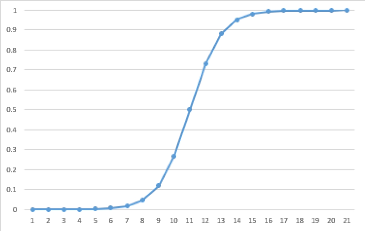
CFL also provides some useful definitions: the parametrized sigmoid function and the Generalized Continuous Linguistic Variable (GLCV). The parametrized generalized sigmoid function is defined by:

It should be mentioned that the sigmoid function has several properties that make it favorable for optimization. First, the function is asymptotic in 1. Because of this, a higher value of x will always have a higher degree of truth. Whereas a non-asymptotic function, such as the trapezoidal, doesn’t recognize increments regarding the value of x within a certain range.

Second, the asymptotic nature of the sigmoid function complies with the notion of Pareto dominance because a non-dominated solution will always have a higher degree of truth than the solutions it dominates (the better the objective value, the higher degree of truth). Using Equation 3, CFL is able to define the parametrized GLCV as follows [⁶]:

Each GLCV has three parameters that modify its behavior: α is used to express the level of tolerance of variations in x. A high value of α is used to indicate that the tolerance is low, whereas a lower value would indicate a higher level of tolerance. γ is used to define the magnitude of x at which the truth value of the GLCV is 0.5, while m is used to determine the behavior of the function. With m=1, the GLCV will behave like a sigmoid function, as depicted in Figure 1, which expresses the maximization of the input variable.

Fig. 1 GLCV as a sigmoid function 

On the other hand, m=0 will make the GLCV behave like an inverse sigmoid, as depicted in Figure 2, which expresses minimization. Using GLCVs, we are able to create CFL predicates like the one described in Equation 5:

Fig. 2 GLCV as an inverse sigmoid function 

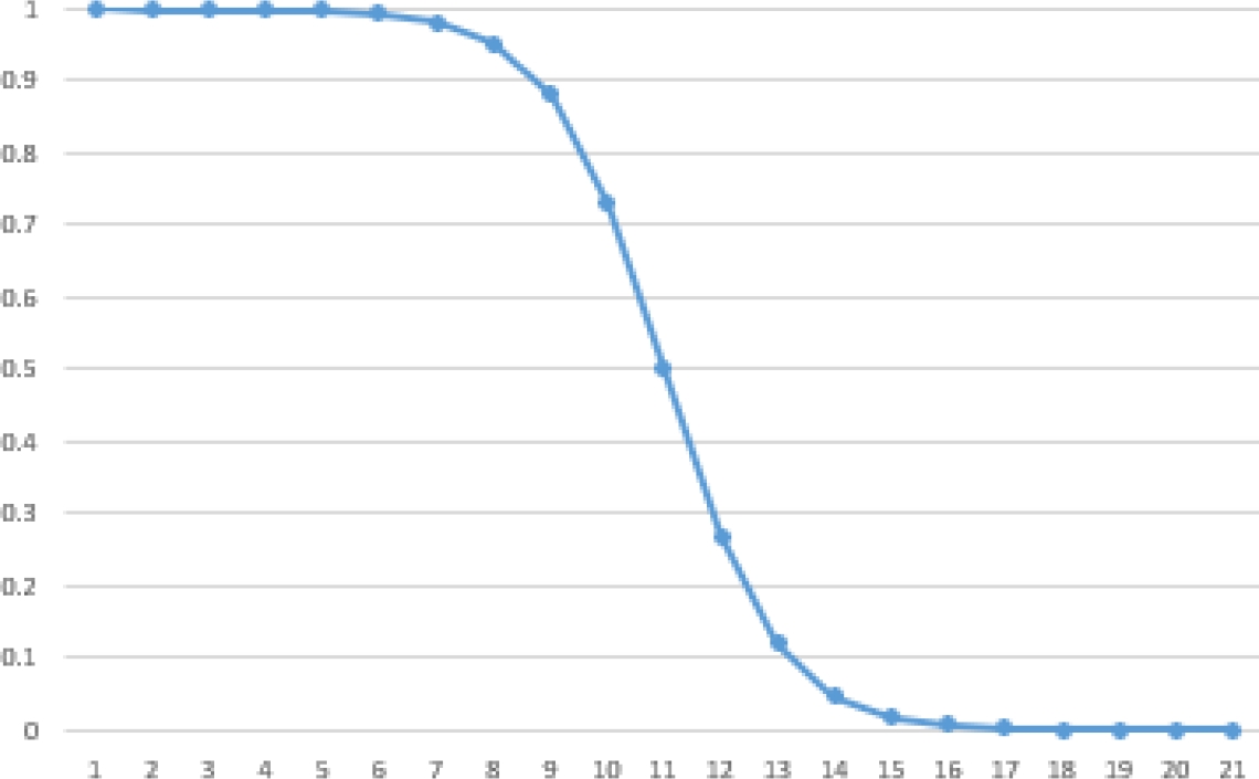
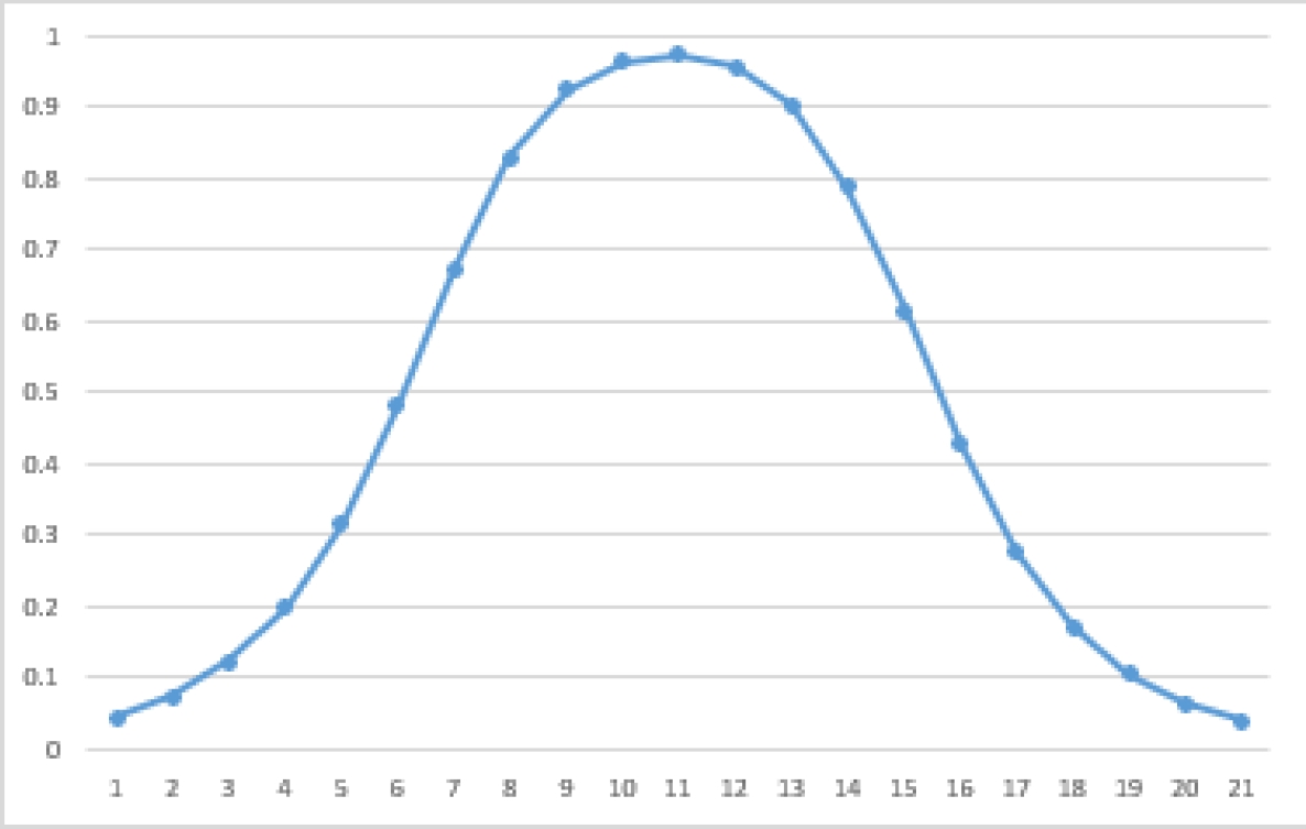
The predicate will behave as a sigmoid function if all of the GLCVs are sigmoids, as an inverse sigmoid if all of the GLCVs are inverse sigmoids, and as a concave function if some GLCVs are sigmoid and others inverse sigmoid. The last case is depicted in Figure 3.

Fig. 3 CFL conjunction predicate 

4 Proposed Model

To create a test instance, we selected 14 indexes pertaining to the Mexican Stock Exchange. The mean return value for each index was calculated using the daily value at the beginning and the value at the cut from 2021 to 2022.

Then, those indexes with negative returns were discarded. Our proposed model employs the GLCV [⁶] to create fuzzy predicates that reflect the investor’s preference.

4.2 Particle Swarm Optimization

PSO is a population-based heuristic used to solve optimization problems. The optimization process is depicted in Figure 4. The first step is used to initialize the swarm. This involves creating a new PSS solution for each particle. Within the PSO, we refer to the solution assigned to the particle as its position.

Fig. 4 Optimization process 

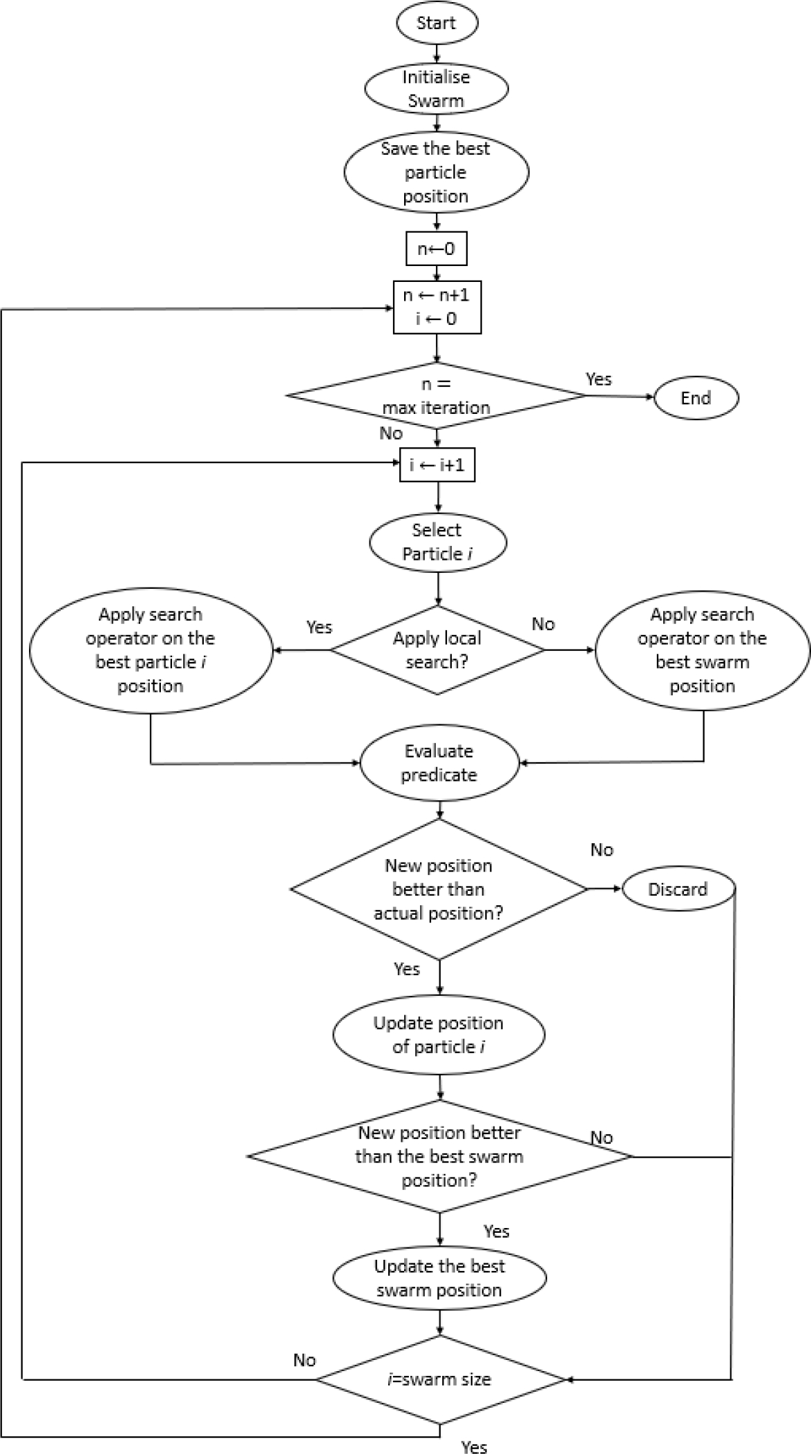
Then, all particles are evaluated by the objective function, the CFL predicate, and the best particle position is saved as the best swarm position. After this step, the optimization process begins.

This process starts by choosing whether the search operator will be applied to the best swarm position or to the best solution found by the particle so far. This selection is done with Equation 9:

xi(t+1)={s(p,v)     ifR1ap>R2ag,s(g,v)     ifR1ap≤R2ag, (9)

Here, xi(t+1) denotes the next position of the particle, R1 and R2 are random numbers in the range [0,1], while ap and ag are the acceleration constants. Lastly, v is the velocity constant.

The mentioned constants modify the behavior of the swarm. The acceleration ones are used to favor either the selection of the best position of the particle or the best position of the swarm. The velocity constant indicates how many times the search operator is applied.

After creating this new position, the objective function will be used to evaluate it. If the new position is not better than the previous position, it is discarded, and the iteration ends. Whereas if the new position is better, it replaces the current position. Lastly, the position is compared with the best swarm position.

If it is better, it will also replace it, and the iteration ends. This process will continue until PSO reaches the maximum number of iterations previously set by the user.

4.2.1 Solution Coding

To represent each portfolio, we used a float array where each number represents the percentage of the budget to be invested for index i. In Figure 5, we show an example of a solution for the test instance. In Figure 5, we can appreciate how one of the indexes has 0% of the budget. This is an acceptable case within our PSS model, as well as one index having the whole budget.

Fig. 5 Portfolio example 

4.2.2 Search Operator

The search operator creates a new solution from a given solution. To do this, the operator randomly selects an index xi with a budget percentage over 0%. After selecting the index, a percentage p between 1% and 100% is randomly set to extract from xi. Then, the extracted budget is added to a random index xj.

To illustrate the operator, we will apply it to the portfolio shown in Figure 5. First, x1 is randomly selected. Then, p is randomly set at 25%, corresponding to 0.05 of the budget percentage assigned to x1. After that, x5 is randomly selected to receive the 0.05 from x1.

The budget is assigned to x5 and extracted from x1, resulting in the solution shown in Figure 6. Since the operator bases the budget exchange on percentages, there is no need to satisfy any budget constraint.

Fig. 6 Modified portfolio 

4.2.3 Initial Swarm

To create the first swarm, each solution is created by assigning equally the budget to each index. The percentage is calculated by 1/a, where a is the number of indexes to consider. The result is truncated to two digits. Because of the nature of this operation, it is possible that the total budget could be less than 1.

To correct this, we simply determine the missing budget and randomly assign it to an index. In Figure 7, we show how a solution is created using this method where the number of indexes is 6.

Fig. 7 Solution adjustment 

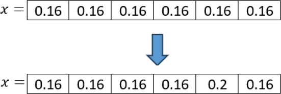
As shown in Figure 7, each index is assigned a budget percentage of 0.16 in the first step. However, when calculating the total budget for this solution, the result is 0.96. Because of this, the remaining 0.04 to reach 1.0 is randomly assigned to the 5th index.

After creating the first solution, the PSO will use it to create the initial population. This is done by applying the local search operator to the initial solution to create each particle. In Figure 8, we show an example of this process.

Fig. 8 Initial population 

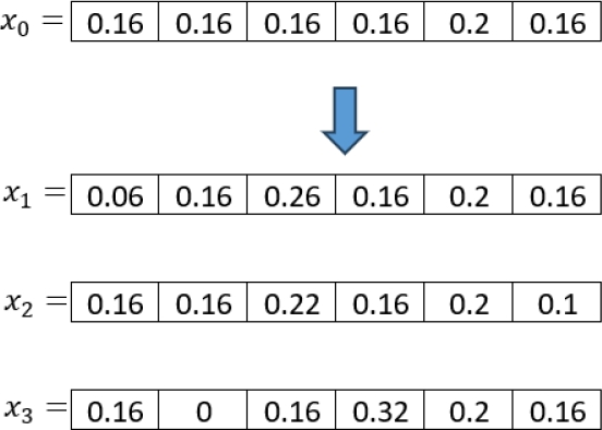
Because this is the first solution for each particle, it is set as the best personal solution found so far. Each particle is evaluated using the objective function. An implementation of the proposed model is available at GitHub^fn.

5 Results

To determine the ability of the proposed model to implement multiple preferences, we defined three investor profiles. The first one, Ia, is an aggressive investor, meaning that it will prioritize a higher return over the risk. Second, Ic is a conservative investor that prioritizes a low risk. Lastly, Ib is a balanced investor seeking an advantageous trade-off between risk and return. The model was coded in Python 3, and all experiments were run on a Windows 10 PC with 16GB of RAM and a 3.9 GHz CPU. All of the investor profiles will use two portfolios as references. One with high return and one with low risk.

In practice, an investor should have this knowledge a priori. The values employed for our experiments are shown in Table 2. Using these values as a reference, we can initialize the fuzzy parameters for each investor profile. In the case of γ, we simply need to indicate a reference value between the highest and lowest value to indicate where the investor assigns a 0.5 level of satisfaction.

For the value of α, we first need to indicate a reference value where the investor assigns the 0.99 level of satisfaction. Once γ is defined, we use Equation 3 to isolate α; this equation is used because of the generalized sigmoid function used within the GLCV:

Here, x denotes the reference value. It should be noted that while calculating α for the risk GLCV, we use −α to reflect its minimization. We selected the reference values for each profile based on a given percentage for each profile. The percentages used for each profile are shown in Table 3.

As shown in Table 3, all investors have an α of 99%. This indicates that every investor will have the maximum truth value on the highest return value and the lowest risk value. In the case of the aggressive investor, we see that the γ point will be 90% close to the highest return value and 70% to the lowest return value.

This means that this investor will only assign values above 0.5 to the highest return portfolios while allowing the portfolio to have a higher risk. In contrast, the conservative investor will only assign values above 0.5 to those portfolios that are 90% close to the lowest risk while allowing the return to decrease.

5.1 Parameter Tuning

To assess the performance of the preference model, we ran a series of experiments with different PSO velocities and acceleration constants using a swarm of 50 particles for 120 iterations. The test values are shown in Table 4. Each combination of parameters was run 30 times. The average truth value of the predicate for each combination is shown in Table 5.

Table 4 Test parameters 

Parameter	Values
Velocity constant	10	5	1
Acceleration constant p	1	1.5	2
Acceleration constant g	1	1.5	2

Table 5 Parametric results 

Combination	Ia	Ib	Ic
1	0.5407	0.6604	0.5513
2	0.9667	0.9715	0.9244
3	0.9712	0.8765	0.9062
4	0.8057	0.8059	0.7817
5	0.9972	0.9917	0.9937
6	0.9432	0.9652	0.9583
7	0.9410	0.8214	0.8615
8	0.9002	0.9878	0.9597
9	0.9927	0.9810	0.9847
10	0.2085	0.3331	0.2580
11	0.9172	0.9177	0.9000
12	0.9173	0.7654	0.8195
13	0.6307	0.5604	0.5987
14	0.9916	0.9361	0.9671
15	0.9247	0.9172	0.9210
16	0.8160	0.7692	0.7362
17	0.9990	0.9917	0.9947
18	0.9795	0.8613	0.9360
19	0.1512	0.1593	0.1473
20	0.8201	0.7508	0.7533
21	0.7003	0.6167	0.6405
22	0.4322	0.3710	0.4282
23	0.9297	0.8783	0.8793
24	0.9303	0.8280	0.8396
25	0.5272	0.5540	0.5329
26	0.9908	0.9755	0.9705
27	0.9708	0.9104	0.9303

Table 5 identifies combination 17 as the best and combination 19 as the worst. Combination 17 has the values of velocity =5, p=1.5, and g=2. Combination 19 has the values of velocity =1, p=2, and g=1. In Figure 9, we can see the non-dominated solutions regarding combination 17.

Fig. 9 PSO results on combination 17 

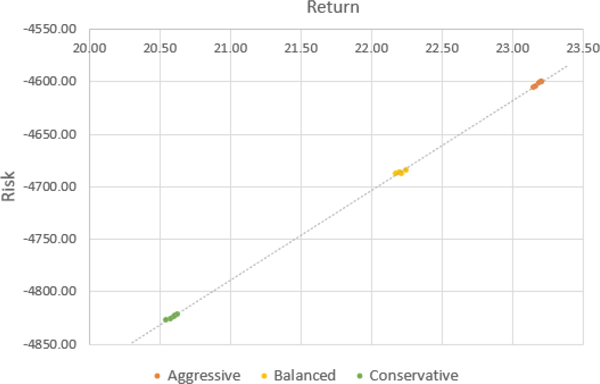
Figure 9 shows how the profile solutions reflect the desired preference. The aggressive profile obtains solutions that have the most return and risk, while the conservative profile favors those solutions with lower return and risk, and the balanced profile is between the two.

These results are achieved due to the fuzzy parameters of Equation 8. The parameters set for the aggressive profile evaluate the solutions belonging to the conservative profile with a lower truth value and vice versa.

Only those solutions that align with the preference reflected by the fuzzy parameters will be assigned a high truth value. This guides the PSO to the desired Pareto-efficient solutions.

6 Conclusions and Future Research

In this paper, we proposed a preference model based on Compensatory Fuzzy Logic (CFL) to solve the Stock Portfolio Selection (PSS) problem. Using CFL, we were able to create predicates that expressed an investor’s preferences regarding the return and risk of the desired portfolio.

These predicates are composed using sigmoid linguistic variables linked with CFL logical operators. The sigmoid function is selected because of its asymptotic properties that allow for a finer evaluation of a variable.

We integrated this model into a Particle Swarm Optimization (PSO) algorithm and ran a series of experiments with three investor profiles using data from the Mexican Stock Market. First, we did a parameter tuning experiment that revealed the best and worst PSO parameter values regarding the truth value of the CFL predicate.

The results suggest that the performance of the PSO is at its best when the swarm slightly favors global search with a medium velocity. In contrast, the worst performance corresponds to a swarm that has the minimum velocity and greatly favors local search.

Using the best combination of parameters, we see how the preference model consistently reflects the preference of each investor profile. It should also be noted that we in order to adjust to each investor profile, we only need to modify the parameters of the linguistic variables that form the CFL predicate.

We made a comparison based on the solutions obtained with PSO without the use of the CFL predicate during the optimization process and the solutions obtained by using CFL predicates. Investor profiles were created based on both results. Then, every solution was evaluated using both sets of investor profiles.

The results showed that the investor profiles obtained by using the CFL predicate during the optimization process have a higher truth value. The Mann-Whitney-Wilcoxon test showed that there were significant statistical differences between the two sets of solutions.

The main limitation of the model is that it needs to have information about the desired solution. Therefore, an investor unfamiliar with the possible outcome in terms of risk and return would not be able to initialize the CFL predicate properly.

For this reason, as future research, we propose the integration of an interactive module within the optimization process. This module should interact with the investor by presenting information about the found solutions and adjusting the sigmoid functions and the CFL predicate based on the investor’s preferences. Another topic for future research is the use of another instance using indexes belonging to other markets. We also propose the implementation of the CFL predicate within a more complex heuristic, such as [¹¹].