


 nova página do texto(beta)
 Inglês (pdf)
 Artigo em XML
 Referências do artigo
 Enviar este artigo por email
 Citado por SciELO
  Similares em
SciELO
Similares em
SciELO 
 Permalink
1. Introduction
The study of scattering problems are very interesting and have lead to important discoveries in many areas of physics such electrodynamics, classical mechanics and quantum physics [1]. In particular, resonant scattering of particles or waves allows the detailed understanding of the inner structure of a system through the analysis of their eigenmodes and its distribution, as has been done in classical wave cavities, microwave graphs, quantum dots, optical microcavities, nucleus, atoms and molecules, to mention just a few.
A simple general model to study resonant scattering consists of a one-mode single port terminal connected to a system of arbitrary complexity; although simple, this general model serves well to explain the main physical features of resonant scattering of more complex systems. A particular case considers an Aharonov-Bohm ring, a single loop that encloses a magnetic flux, that is connected to a reservoir through a straight terminal. This system preserves the simplicity of one-dimensional problems since it enables a wide analytical study but, in a very important manner, introduces the tuning of the scattering process in two ways, the interplay of the coupling of the ring with the terminal, and the phase due to the Aharonov-Bohm effect.
The loop connected to a port has been considered from several perspectives, many of them related to electronic transport in normal metal rings. In this way, it has been very useful to understand the relations between the scattering matrix, persistent currents, and magnetoresonances [2-4], as well as to analyze the effect of a reservoir [5], or the absorption by a inductively coupled heat load that occurs during the measurements of these currents [6]. More recently, technological advances in the fabrication of nanostructures have renewed the interest about magnetic properties of quantum rings, made of semiconductors or graphene [7-9], or by the advent of the molecular elctronics [10].
In this paper we revisit this model, loop or ballistic ring pierced by an Aharonov-Bohm flux, while being feed by means of a single mode ballistic wire. Our purpose is to analyze the effect of the magnetic flux on the phase, the Wigner delay time, and in the wave function in general. More precisely, we look for the effect of the magnetic flux on the distribution of the phase of the scattering matrix along the unitary circle in the Argand plane, whether this distribution is given by the so called Poisson kernel, as well as its relation to the Wigner delay time; we also ask for the distribution in energy of the Wigner delay time and how it is affected by the magnetic flux.
2. Scattering properties of a resonant system
Any scattering problem by a potential of finite range can be described by a scattering matrix, usually denoted by S, which is obtained by solving the Schrödinger equation. By definition, S relates the outgoing plane wave amplitudes to the incoming ones and, for a problem of N open modes (or channels), S is a N ×N unitary matrix, unitarity being due to flux conservation [11].
Since S contains all the information about the system due to the scattering potential, physical observables can be obtained from it; we restrict ourselves to two properties. For example, unitarity of S implies that its determinant, det S, is a complex number of modulus 1, which describes a circle in the Argand plane when the energy E of the incident particles is varied. The phase of this complex number, denoted by θ, is known as Friedel phase [12, 13]. In particular, for the one-channel case, N = 1, the complex number is exactly the scattering matrix (we are interested in the single mode case), namely
in fact θ(E) is twice the phase shift plus π [11]. Another important observable is the Wigner time delay (see Ref. [14] and references there in), which for N = 1 is defined as the derivative of θ with respect to E [11, 15],
In the optical model [16, 17] the amplitude of the scattering wave consists of the sum of two contributions, one coming from the prompt response, direct processes, while the other leaves the system after a delay. The prompt response corresponds to a smooth behavior of the scattering matrix that is independent of the energy, E, and it is quantified by the energy average of S over a sufficiently large interval, denoted by 〈S〉 and referred to as the optical S-matrix. Therefore, S can be splitted as [11]
where S d(E) represents the delayed part. The absence or presence of direct processes has drastic consequences in scattering properties, in particular in how the scattering matrix visits its available space as E is varied. This is what we will refer to as a distribution, not associated to a random process (although it could be by appealing an ergodic hypothesis). In the former case, S visits its space in a uniform way, such that 〈S〉 =0, while in latest one S distributes according to the Poisson kernel. For instance, for N = 1 it is given by [11, 18]
An interesting feature of this distribution is that it is univocally determined once the parameter 〈S〉 is given, unless there is dissipation or gain [19]. If 〈S〉 = 0, p 〈S〉 (θ) reduces to a constant, if not, the phase θ does not visit uniformly the circumference of the unit circle. A demonstration of the Poisson kernel uses an analyticity condition which implies that 〈S n 〉 = 〈S〉 n , with n an integer. For many problems, 〈S〉 is obtained from experimental data, but in recent investigations it is given by the problem itself [20,21]. Moreover, a physical realization of the Poisson kernel is artificially constructed by assuming a model for the coupling of the scattering region to the external world [22, 23].
3. Resonant scattering in a ring pierced by a magnetic flux
The system consisting of a single mode ballistic ring of radius R, pierced by a magnetic flux Φ, is shown in Fig. 1. The ring is coupled to a single mode ballistic wire through a junction whose scattering potential is described by a fixed scattering matrix S 0. For simplicity, we assume that S 0 is a real symmetric matrix, namely [24]
where 0 ≤ 𝜖 ≤ (1/2),
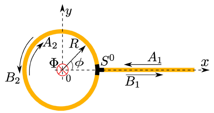
Figure 1 (Color online) Single mode Ballistic ring of radius R pierced by a Aharonov-Bohm flux Φ, indicated by a filled circle inside (red), feeded by a single mode ballistic wire. The coupling between ring and the wire is indicated by a T-junction in black, whcih is described by a fixed 3 × 3 scattering matrix S 0. A 1 and B 1 represent the amplitudes of the incoming and outgoing plane waves in the wire, respectively, while A 2 and B 2 represents the plane wave amplitudes into the ring, traveling counter clockwise and clockwise direction, respectively; ϕ is the angle in the counter clockwise direction.
Assuming that the ring is on the xy plane, the wire along the x axis and the coordinate system at the center of the ring, as shown in Fig. 1, the junction is placed at x = R such that the solution of the Schrödinger equation along wire can be written as [3]
where k is the wave number,
where ϕ is the azimuthal angle; A 2 and B 2 are the clock-wise and counterclockwise plane wave amplitudes, respectively. ψ 2(ϕ) satisfies unusual boundary conditions [25]: ψ 2(2π) =ψ 2(0)e i2πφ , where φ is the magnetic flux in units of the flux quantum or fluxon, φ = Φ/(h/e) (in SI units).
3.1. Solution of the scattering problem
By definition, S 0 relates the outgoing amplitudes to the incoming ones at the junction, as [3]
where L = 2πR, is the perimeter of the ring. This matrix equation can be solved for B 1 in terms of A 1 to give
where S is the 1 × 1 scattering matrix of the system. Using the model for S 0, Eq. (5), the resulting scattering matrix of the system can be expressed as
where I
2 stands for the 2 × 2 unit matrix. Here,
and
Similarly, Eq. (8) can be solved for A 2 y B 2 in terms of A 1; the result is
3.2. Bound states
The bound states are obtained for the closed system, when the ring is decoupled to the wire. For ϵ =0, Eqs. (5) and (8) gives B 1 = -A 1, such that wave function in the wire the becomes
once the amplitude A
1 is chosen properly as
These values of k imply discrete energy values that depends quadratrically on φ [26].
3.3. Resonances
The 1×1 scattering matrix of Eq. (10) is just a complex number of modulus 1, as in Eq. (1); explicitly, we have
that shows the dependence of S on φ and k explicitly. Therefore, due to flux conservation, the motion of S in the Argand plane describes a circle of radius 1. This is shown Fig. 2, panels (a) for φ = 0 and (d) for φ = 0.3.
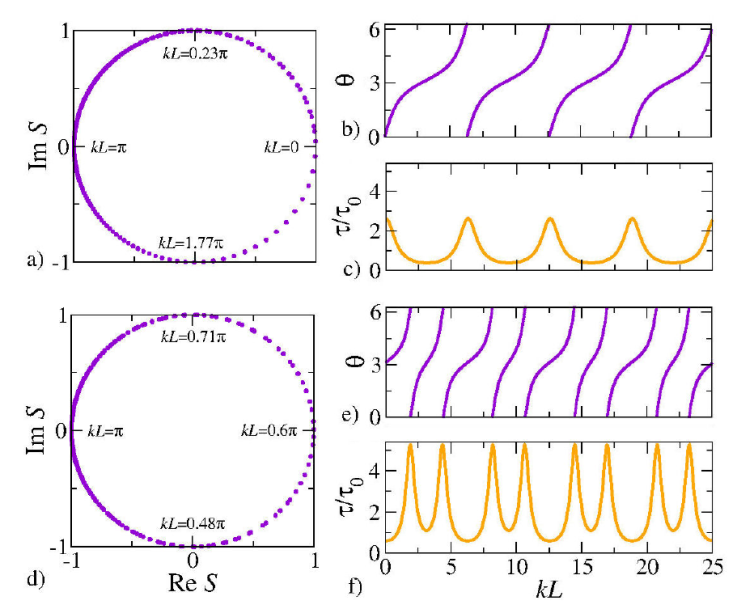
Figure 2 For 𝜖 = 0:4 we show: Motion of S(kL) in the Argand plane for a) φ = 0 and d) φ = 0.3; phase θ(kL) for b) φ = 0 and e) φ =0.3; Wigner time delay, in units of τ 0, for c) φ = 0 and f) φ = 0.3. For instance, S(2πφ) = 1 and S(π) = -1, S(0.23π) = i and S(1.77π) = -i for φ = 0, while S(0.48π) = -i and S(0.71π) = i for φ = 0.3.
It is convenient to write θ = 2- + π, where δ is the phase shift given by
From this expression we observe that an abrupt change in
δ(k), and hence in
θ(k), occurs at
The resonances are also exhibited in the Wigner time delay; it is easily obtained from the definition (2), namely [3]
where τ 0 = L/(ħk/M), which is the time that the particle takes to travel freely the circumference of the ring. Equation (18) shows the dependence of τ on φ and k explicitly. The behaviour of τ (k) is also shown Fig. 2, in panels (c) for φ = 0 and (f) for φ = 0.3, where each resonance is clearly observed as a local maximum.
In Fig. 2c), we may observe that for φ = 0 the resonances are isolated and symmetric with respect to its center, located at
The shape of the resonance can be determined analytically making an expansion close to a resonance in a weak coupling limit. The result is
for φ ≠ 0, which is a typical Breit-Wigner form of a resonance of width 𝜖, centered at kL = 2πφ + 2nπ. For φ = 0, the result is
a resonance of width 2𝜖, centered at kL = 2nπ.
3.4. Wave function at resonance
The wave function in the wire can be obtained by substitution of S = -e
2iδ
into Eqs. (9) and (6). Once the normalization constant is chosen to be
which is similar to that of Eq. (14), except for the phase shift δ. Similarly, substitution of amplitudes A 2 and B 2 from Eq. (13) into Eq. (7), gives the wave function along the ring,
where
The evaluation of the wave function at a specific position in the ring is shown in Fig. 3, in its square modulus times R, as a function of kL for 𝜖 = 0.4 and φ = 0.3. The resonance peaks are clearly observed. The shape of the resonances can also be obtained making an expansion for kL very close to
for φ ≠ 0, and
for φ = 0. Again, these resonances are of the Breit-Wigner form and are the same of those of Eqs. (19) and (20), as should be.
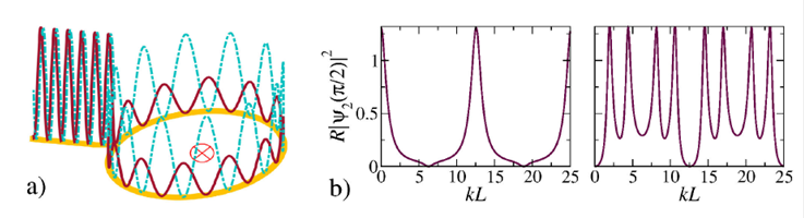
Figure 3 Square modulus of the wave function, times R, for 𝜖 = 0.4. a) Spatial behaviour for φ = 0 (cyan discontinuous line) and φ = 0.3 (magenta continuous line). b) The behaviour at ϕ = π/2 in the ring, for zero flux (left) and φ = 0.3 (right), shows the resonance peaks when it is plotted as a function of kL.
4. Probability distributions
It has been noticed that S describes a circle of radius 1 as the energy of the particle is varied, see Fig. 2a) and d). In the same figure we can also observed that S does not visit the circumference in a uniform way. In this section we address the distribution of the phase of the scattering matrix in the Argand plane and establish a relation with the Wigner delay time. At the same time, we determine the distribution of this last quantity.
4.1. Probability distribution of the phase
The scattering matrix of the system, given by Eq. (10), can be directly written as
This expression is of the form of Eq. (3); it is easy to identify the optical matrix as
Therefore, it is expected that the distribution of the phase θ along the circumference is give by Poisson’s kernel, Eq. (4).
In Fig. 4 the histogram of the phase θ for two resonances, for φ = 0 and φ = 0.3, is compared with the Poisson kernel distribution, Eq. (4), with 〈S〉 given by Eq. (26). In Fig. 4d) we observe that the Poisson kernel describes the distribution of the phase for φ = 0, while it does not for φ = 0.3. It is worth to note a symmetry in the shape of an isolated resonance in the phase: it is invariant under two reflections, one with respect to a vertical line at the resonance in the kL-axis, followed by a second reflection with respect the horizontal line θ = π. This symmetry is absent for φ = 0.3. As a consequence, a deviation with respect to Poisson’s kernel at θ = π is observed in the distribution of θ in Fig. 4e): the values of θ just below θ = π becomes depopulated but populated just above of it. Poisson’s kernel is recovered if an interval of 2π in kL contains the two overlapped resonances, Figs. 4c) and 4f).
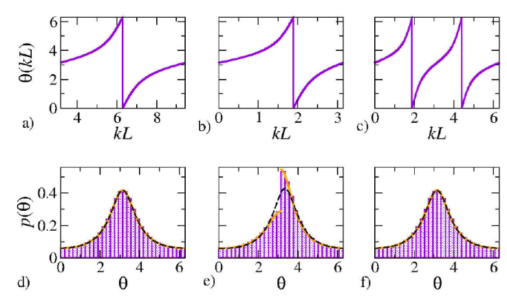
Figure 4 Phase θ and its distribution p(θ) for 𝜖 = 0.4: a) and d) for φ = 0 and resonance at kL = 2π; b) and e) for φ = 0.3 and resonance at kL = 0.6π; c) and f) for φ = 0.3 and resonances at kL = 0.6π and kL = 1.4π. The bars in d), e), and f) are the histograms obtained from the phase θ(kL) of panels a), b), and c); the discontinuous (black) lines correspond to Poisson’s kernel, while the continuous (orange) lines are the reciprocal of the time delay.
The reciprocal of the Wigner delay time is also plotted in Fig. 4, as an implicit function of θ through its dependence on kL, for the corresponding resonances of panels 4a) for φ = 0, 4b) and 4c) for φ = 0.3. The excellent agreement with the respective histograms says that the reciprocal of the Wigner delay time describes exactly the distribution of the phase. It is concluded that
where C is a normalization constant: C = 1/2π for φ = 0, while C = 1/π for φ = 0.3. We accentuate that the dependence of τ/τ 0 on θ is implicit through kL. That is, an explicit determination of τ/τ 0 as a function of θ requires the inversion of Eq. (25) to write kL in terms of θ and substitute into Eq. (18). The result reduces to Eq. (4) with 〈S〉 given by Eq. (26). However, this procedure is not necessary since Eq. (27) is easily demonstrated, as is shown in what follows.
The Wigner time delay, as it is defined in Eq. (2), can be written in terms of the wave number k, or kL, for the particular case of the the ring, as
As sugested by Fig. 4, we assume a uniform distribution for the variable kL and establish the equality of the probabilities for the transformation θ = θ(kL); that is
where C is the normalization constant of the uniform distribution of kL. Therefore,
which using the last equality Eq. (28) lead us to the result of Eq. (27).
This prodecedure is important since it enables to determine the distribution of the Wigner delay time.
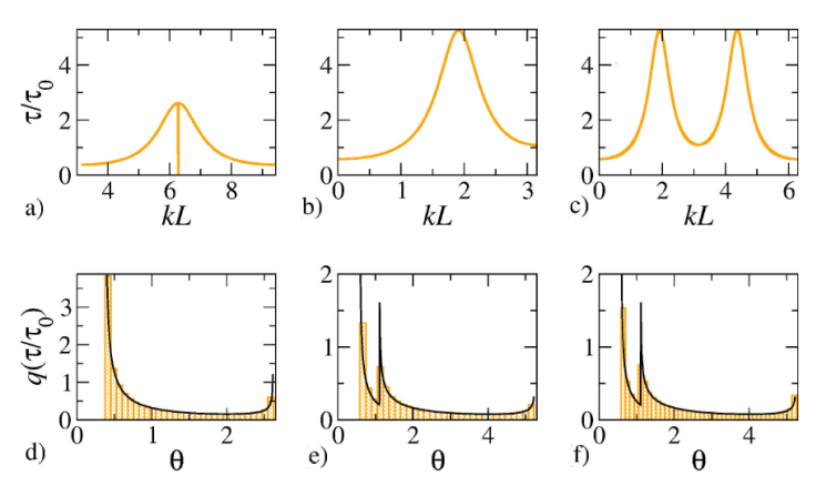
4.2. Probability distribution of the Wigner delay time
It is also interesting to look for the distribution of the Wigner delay time delay. Lets define y ≡ τ/𝜖τ 0, such that
Therefore, if q ’ (y) is the probability density distribution of y, the corresponding one for τ/τ 0 is q(τ/τ 0).
Since the probability is invariant under the transformation y = y(kL) and that kL is uniformly distributed, then
from which
From Eq. (18) we find that
where
Now, from Eq. (31),
and
with A given by Eq. (35). Note that both signs (±) correspond to different branches of the Wigner delay time around the resonance. For symmetric resonances, like that for φ = 0, the right sign is (+) and C = 1/2π, while for non-symmetric resonances, the sing (-) corresponds to the left branch and the (+) sign to the right branch of the resonance; C = 1/π for the whole interval of the two overlapped resonances.
Finally, the probability density distribution of τ/τ 0, for φ ≠ 0, is given by
where Θ(x) is the Heaviside function and q± (x) is given by
with
Equation (38) is not valid for φ = 0, 1/2, for which the distribution of the time delay should be calculated separately; for these cases,
where A 0 is A φ for φ = 0. In Fig. 5 the distribution of the Wigner delay time for the same resonances as in Fig. 4, for φ = 0, 0.3, are shown and compared with the analytical results; the observed agreement is excellent. We also note that for φ = 0 there is a set of zero measure just at the resonance kL = 2π for which τ = 0.
5. Conclusions
We have studied a simple but general model to study the effect of quantum scattering, a ring pierced by a static magnetic flux, coupled to a wire has been used to analyze the influence of the magnetic flux on the distributions of the phase and the Wigner delay time. It is well known that for zero magnetic flux and specific values of it, the resonances are isolated; for any other values of the flux they become overlapped by pairs, each one being non symmetric. We established a relation between the motion of the 1 × 1 scattering matrix in the Argand plane and the Wigner delay time. For a single non overlapped resonance, or two overlapped resonances, the Poisson kernel describes the distribution of the phase; the effect of the magnetic flux is implicit through the value of the optical matrix. What is new here is our finding that Poisson’s kernel coincides with the reciprocal of the Wigner delay time. Of course, this result is not valid when only one of the overlapped resonances is taken into account, because the lack of symmetry in the shape of single resonances. Our findings provides a new interpretation of the Wigner delay time: besides of being the lapse of time taken by the interaction of the particle with the scattering potential, it is now also interpreted as the rate of occurrence of a phase in the unit circle, while the wavenumber moves with a constant step. It should be interesting to verify whether this holds for a scattering matrix of larger dimensions.
Appealing to a similar interpretation of a probability distribution, and following the same procedure for the phase, we were able to determine the distribution of the Wigner delay time. Contrary to the distribution of the phase, the distribution of the Wigner time delay exhibits explicitly the effect of the magnetic flux, independently whether one or two resonances are considered.

