SciELO - Scientific Electronic Library Online

 
vol.25 número4Validación de una microrred mediante software in the loop para la inyección de potencia activa en redes eléctricas de distribuciónModelación mediante PWC debido a la presencia de plaguicidas organoclorados en los canales de Ampampilco y Apatlaco, Xochimilco índice de autoresíndice de materiabúsqueda de artículos
Home Pagelista alfabética de revistas  

Servicios Personalizados

Revista

Articulo

Indicadores

Links relacionados

  • No hay artículos similaresSimilares en SciELO

Compartir


Ingeniería, investigación y tecnología

versión On-line ISSN 2594-0732versión impresa ISSN 1405-7743

Ing. invest. y tecnol. vol.25 no.4 Ciudad de México oct./dic. 2024  Epub 08-Abr-2025

https://doi.org/10.22201/fi.25940732e.2024.25.4.031 

Articles

Intelligent iPD control estimation of Hardware-in-the-Loop generated dynamics

Control inteligente PD de dinámicas generadas con Hardware-in-the-Loop

Juan Carlos Martínez-García1 
http://orcid.org/0000-0003-2931-0531

Alberto Soria-López2 
http://orcid.org/0000-0002-6310-9527

1Instituto Politécnico Nacional. México, Centro de Investigaciones y Estudios Avanzados, Departamento de Control Automático E-mail: juancarlos.martinez@cinvestav.mx

2Instituto Politécnico Nacional. México, Centro de Investigaciones y Estudios Avanzados, Departamento de Control Automático E-mail: soria@cinvestav.mx


Abstract

Hardware-in-the-Loop (HIL) perturbation load generated dynamics are estimated using an intelligent Proportional Derivative (iPD) control. Our contribution is show real-time results on how the iPD estimates explicitly the unknown dynamics term, allowing a better knowledge the way in which iPD works, whereas in the related literature, only simulation results have been presented without clearly showing the estimated term that is at the core of the iPD control. The intelligent iPD is a particular intelligent control scheme, unlike intelligent control that uses fuzzy logic, neural networks or genetic algorithms, the unmodeled dynamics are approximated by integrals reducing real-time system measurements noise in the control loop and implemented using a Finite Impulse Response (FIR) digital filter. We use two DC servo motors interconnected by their shafts. The first DC servo motor is controlled by the proposed feedback-based iPD controller whereas the second DC servomotor is used as a programmable torque load to the controlled DC servo motor. Using HIL testing we can generate desired unknown load torques for the controlled servomotor directly showing how the iPD controller approximates HIL generated perturbations. For the proposed control iPD scheme, we present both computer-based simulation and experimental real-time control results.

Keywords: Intelligent iPD control; modeling and control; dc servomechanisms; real-time control

Resumen

Las dinámicas de perturbación de carga se generan usando Hardware-in-the-Loop (HIL) y se estiman empleando un esquema de control Inteligente Proporcional Derivativo (iPD). Nuestra contribución es la presentación de resultados experimentales en tiempo real para mostrar cómo el iPD estima el término de la dinámica desconocida para el servomotor controlado, permitiendo un mejor conocimiento del funcionamiento del iPD mientras que en la literatura asociada, y solamente en simulaciones, no se ha presentado claramente el término estimado que es esencial en el control iPD. El iPD es un esquema de control inteligente particular, a diferencia del control inteligente que utiliza lógica difusa, redes neuronales o algoritmos genéticos, la dinámica no modelada se aproxima mediante integrales que reducen el ruido de las mediciones del sistema en el lazo cerrado y se implementa mediante Filtros de Respuesta Finita al Impulso (FIR). Se propone el uso de dos servomotores de corriente directa (CD) interconectados por sus ejes. El primer servomotor utiliza el controlador iPD, mientras que el segundo servomotor se utiliza como una carga programable de la dinámica no conocida para el servomotor controlado.

Descriptores: Control inteligente iPD; modelado y control; servomecanismos de CD; control en tiempo real

Introduction

The model-free Intelligent PID controller or iPID controller was introduced by Fliess, Join, Mboup and Sira-Ramírez in Join et al. (2006) and Fliess et al. (2006a and b) taking into account unknown dynamics of the plant by using an ultra-local model approach without any modelling procedure. The iPD uses an online numerical algebraic differentiator (Fliess & Sira, 2003; Mboup et al., 2007) to estimate the plant unknown dynamics implemented as an integral filtering a noisy signal. The performance of such a proposed iPID control scheme has been tested for example systems and for models of real systems in simulation as well as for real-time control of physical systems. We shall present only a limited number of references from a much larger number of the published research papers regarding the model-free Intelligent control.

To illustrate the versatility of the model-free iPID control scheme, Fliess, Join and their co-workers applied extensively the model-free intelligent control approach through computer-based simulation. Some references of concerning example systems are an unstable single input single output system (Fliess & Join, 2014); an unstable 3rd order system; a 2nd order delayed system (Doublet et al., 2017); a 2nd order nonlinear system with sign function (Fliess & Join, 2018); a one dimensional heat equation (Fliess & Join, 2018) or a 2nd order linear unstable system (Fliess & Join, 2018). Moreover, Fliess, Join and their co-workers also tested model-free control through computer-based simulation for models of physical systems, for example: a microalgae growth in a closed bioreactor (Tebbani et al., 2016); acute inflammatory response to pathogenic infection (Bara et al., 2016); a freeway traffic flow model (Abouaïsa et al., 2017); a highway multi-ramp inflow traffic regulation (Join et al., 2021) or a multivariable longitudinal and lateral vehicle model (Menhour et al., 2018). In all these applications the model-free control scheme proves its clear advantages over standard model-based PID control. In what follows we shall call iPD control the scheme that consists of an intelligent model-free Proportional and Derivative controller. The intelligent model-free Proportional and Integral control scheme will be just denoted iPI control.

Model-free based control beyond iPID control has also been explored, basically through computer-based simulation. Some examples are: Wang, Tian and their co-workers applied a modified model-free control introducing an adaptation of the model free α parameter for an iPID control scheme with the time-delay estimator (Wang et al., 2020) and adding an adaptive iterative learning compensator and an initial state learning scheme applied to a back-support Exoskeleton (Wang et al., 2021); Chekakta and his co-workers applied a modified iPD controller where the controller gains are tuned using a fuzzy logic system for trajectory tracking of a quadrotor model (Chekakta et al., 2020); Olama and his co-workers applied the model-free approach to control the building end-user power allocation for residential and commercial heating, ventilation, air conditioning and water heater units for a building thermal model in a large-scale power distribution system model (Amasyali et al., 2020); Baciu and his co-workers applied an iPD controller applied an iPD controller for an inverted pendulum system model comparing to a sliding mode controller (Baciu & Lazar, 2020); Elleuch and Damak applied a modified iPD controller combined with a sliding mode control scheme to a robot manipulator model including actuator dynamics (Elleuch & Damak, 2020); Huba et al studied the tuning of iPD controller (Huba et al., 2020); Bembli et al applied a modified iPD control combined with a terminal sliding mode control scheme to an exoskeleton upper limb system model (Bembli et al., 2021); Li et al applied a model predictive current control using an ultra-local model and a sliding mode observer for the estimation to a surface-mounted permanent magnet synchronous motor model (Li et al., 2021); Sehili and Boukhezzar applied an iPID for a direct current motor model (Sehili & Boukhezzar, 2022).

As far as the experimental application of model-free control is concerned, Flies, Join and his co-workers applied for example an iP controller for a greenhouse controlling heating and fogging (Lafont et al., 2014) an iPD controller to drive the pitch, roll and yaw of an acrobatic quadrotor (Clouatre et al., 2020) and both an iPD controller and an iPID controller to a laboratory half-quadrotor (Fliess & Join, 2021).

Other researchers that presented experimental results using the model-free approach, are for example: Ferrari et al. that applied an iP to a diesel-wind microgrid diesel-system model generated HIL dynamics (Ferrari et al., 2021). Han et al. applied an iPD to a 12-dof lower limb exoskeleton replacing the algebraic estimator with a discrete-time extended state observer and computing desired velocities and accelerations with sigmoid function-based tracking differentiator (Han et al., 2020). Quin et al. applied an iPD to a 2-dof laboratory helicopter adding a sliding mode compensator control term and replacing the algebraic estimator with a high pass filter and adding an outer compensation loop using an actor-critic neural network (Quin et al., 2020).

The model-free control approach shows that it is an effective control strategy for a quite wide variety of control applications. However, the estimate of the system unknown dynamics, that play a key role in the control scheme, has received little attention and has only been presented in computer-based simulations. Indeed, Fliess, Join and his coworkers in (Fliess et al., 2006a and b) show the curves for the estimation of unknown dynamics and in (Villagra et al., 2009) the authors show that the estimation, using the algebraic estimator, is closed to the road slope, rolling resistance and aerodynamic force terms; nonetheless it is not clear how these terms where simulated. In this paper we present experimental real-time results to study the estimation of unknown nonlinear HIL generated dynamics using for this purpose a programable load servomotor coupled to a control servomotor.

The rest of our paper is organized as follows, the following section includes a brief presentation of model-free intelligent control including the estimation integrals and the finite impulse digital filter (FIR) coefficients calculation. We then present the HIL servomotor setup, and a nonlinear model used to generate load dynamics. Afterwards we will show the real-time results, finishing with some concluding remarks.

Intelligent iPD control

The data driven intelligent controller or iPD is a control scheme introduced in Fliess et al. (2006a), (Join et al. (2006), Fliess et al. (2006) is based on the ultra-local model:

y(v)(t)=F(t)+αu(t) (1)

Parameter v is the derivation order that in general is 1 or 2. y(t) stands for the output signal of the system, u(t) stands for the control signal, and F(t) denotes unmodeled dynamics. Parameter α is chosen such that when multiplied by u(t) has the same units as F(t).

Using v=2 the iPD control law is given by:

u=-Fest(t)-y¨ref(t)+Kpe(t)+Kde˙(t)α (2)

Where the proportional controller gain K p , the derivative controller gain K d , and α are parameters that are required to be tuned. yreft is the desired reference trajectory. Festt denotes the unmodeled dynamics estimation term. The error is defined as et=y-yref.

Using control law (2) in (1) and considering that Festt-Ft0, the close-loop dynamics are given by:

e¨+Kde˙+Kpe=0 (3)

K p and K d controller gains are selected such that the roots of the corresponding characteristic equation in (3) have strictly negative real parts to ensure that limt+et0.

The unmodeled dynamics estimation term F est as in Fliess & Join (2021), can be approximated taking the Laplace transform of equation (1) considering F est is constant in a small interval, which is to say:

s2Y(s)-sy(0)-y˙(0)=Fests+αU(s) (4)

Deriving twice equation (4) with respect to s, eliminates the initial conditions:

2Y(s)+4sdY(s)ds+s2d2Y(s)ds2-αd2U(s)ds2=2Fests3 (5)

Multiplying both side of equation (5) by s -3 , allows to remove the positive power of s and filter corrupting noise using iterated integrals:

2Y(s)s3+4s2dY(s)ds+1sd2Y(s)ds2-αs3d2U(s)ds2=2Fests6 (6)

The time domain for the right side of (6) is accomplished using the inverse transformation rule:

asr,r1,aCatr-1(r-1)! (7)

The time domain for the left side terms of (6), 1srdng(s)dsn, are obtained as the iterated integral of order r of (-1)ntng(t) using the Cauchy formula for repeated integration based at a. This reduces to the single integral (Mboup et al., 2009):

1srdng(s)dsn1(r-1)!at(t-σ)(r-1)(-1)nσng(σ)dσ (8)

Using equations (6), (7) and (8) with a=t-τ, the unmodeled dynamics estimation F est is approximated with:

Fest(t)=60τ5t-τt(τ2+6σ2-6τσ)y(σ)dσ-30ατ5t-τt((τ-σ)2σ2)u(σ)dσ (9)

The integrals in this equation are implemented (Mboup et al., 2009) using a Finite Impulse Response (FIR) digital filter with impulse response Wkgk given by:

k=0MWkgkxn-k (10)

The weight values W k correspond to Δx k of the trapezoidal numeric integration rule with sampling period T s :

abf(x)k=0MΔxkfk (11)

Where fk=fkTs, Δxk=Ts, k=1,,M-1 and Δx0=ΔxM=Ts2.

Each integral in equation (9) is approximated at time t by:

f(t)=t-τtg(τ,σ)x(σ)dσfn=k=0MWkgkxn-k (12)

In the above equation fn=fnTs, gk=gMTs,kTs and xn-k=xnTs-kTs. FIR filter coefficients are given by bk=Wkgk and the approximation sliding window size and FIR filter order is M and sliding window time size is τ=MTs.

We can at this level present our HIL servo motors setup as well as the corresponding model.

HIL Servo motors setup and model

In Figure 1 we present a picture of the two servo motors coupled by their motor shafts used for the Real-Time experiments. Each servo mechanism includes a direct current (DC) motor, a Peripheral Interface Controller (PIC), a high-speed USB communication microcontroller, a digital magneto resistive isolator, an analog galvanic isolator amplifier, an incremental encoder, an H-bridge and the necessary power supplies for all components. Full details of the servo mechanism, including the system schematic, can be found in González et al. (2018). As software development platform we used Matlab/Simulink (The Math Works, 2012) and the QuaRc (Quanser, 2011). RealTime Kernel with T s =0.0015 sec sampling period. The servo mechanism includes a 10 khz low level current controller allowing the control (or input) signal to be proportional to the torque developed by the DC motor. The peak reference input current, that is the control signal, is limited to [-1,1] amps for the low level current loop PI controller.

Figure 1 Servo motors setup with axle coupling 

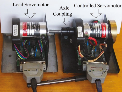
The coupled motor shafts change the controlled servomotor behavior adding friction and inertia. We employ a first order model for the DC motor where parameters are obtained using a closed loop identification method presented in Soria et al. (2010) when output is the speed of motor shaft. We add an integrator to this model to obtain position of the motor:

Y(s)U(s)=G(s)=bs+a1s (13)

If we take v=2 in equation (1) this model in the time domain corresponds to:

y¨(t)=ay˙(t)+bu(t) (14)

Using the identification method mentioned above, we obtained b=94.03 and a=2.45. It should be noted that when first performing the identification of the coupled servomotors, load servomotor input is u HIL (t)=0. Parameter b is related to the amplifier gain and rotor inertia whereas parameter a is related to friction and rotor inertia. Model (14) can be written like equation (1) as:

y¨(t)=F(t)+bu(t)

F(t)=-(αy˙(t)) (15)

When validating model (15) we found that the coupling of the servomotors introduces a perturbation that can be considered adding to model (15) a gravity term:

y¨t=Ft+but

F(t)=-(αy˙(t)+bKintsin( 2πy(t))) (16)

Using the method presented in Garrido & Soria, (2005) to estimate gravity terms, we identified parameter K int =0.1267.

In (16) ut is the controlled servomotor input that is different from the load servomotor input uHIL(t). We proposed real-time load servo motor input signal uHIL(t) that generates the HIL torque as:

uHIL(t)=0.8*sin(2πy(t)) (17)

This torque adds the non-linear term bKHILsin(2πy(t)) to function F(t) in model (16):

Ft=-ay˙t+bKintsin(2πyt+bKHILsin(2πy(t))) (18)

Using method Garrido & Soria (2005) we identified parameter K HIL =0.9013 for the coupled servomotors with HIL torque given by (17).

The proposed model for the servomotors setup with axle coupling includes a friction and gravity terms:

y¨(t)=F(t)+bu(t)

F(t)=-(τint+τHIL) (19)

With τint=ay˙t+bKintsin2πyt and τHIL=bKHILsin2πyt.

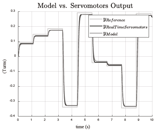
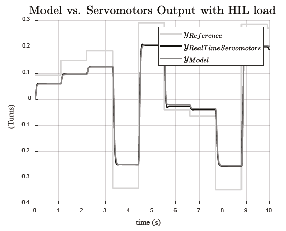
It can be noticed in Figure 3 that the behavior of the real servomotor setup and model (19) are close allowing to confirm that the HIL allows to generate the load torques to the real coupled servomotors.

Figure 2 PD Realtime output vs. model (15) output. τ HIL =0 

Figure 3 PD Realtime Servomotors output vs. model (18) output τ HIL =0 

Simulation and real-time results

We present simulation and real time control results with τHIL=0 and τHIL0. Figure 2 and Figure 3 show model (19) output vs. real-time coupled servomotor output employing the well-known Proportional Derivate (PD) control law, ut=10et-0.6y(t)˙ when τHIL0 and τHIL=0 respectively. We can notice in the PD control, that it does not allow acceptable control results when τHIL=0 and more obviously when τHIL0 where the perturbation load increases the error between the reference and the output.

Estimation of y˙(t) from position measurements and e˙(t) in the control law (2) are performed using a high-pass filter to approximate the derivatives:

G(s)=s350s+350 (20)

In the simulation and the real time results we manually tuned the required parameters as in most of the published literature about iPD control, setting sliding window size M=80, α=94.03, Kp=710.59 and Kd=39.81. The controller gains were tuned for τHIL=0, and where not changed for τHIL0 allowing to perceive how the estimation used by the controller performs when the controller gains are not tuned for a higher load.

Figure 4 shows the control results when τHIL=0; the model follows the reference signal more closely than in real-time having a smaller error signal as shown in Figure 10. Figure 5 shows the control results when τHIL0; the model follows the reference signal more closely than in real-time having a smaller error signal as shown in Figure 11. Control signals are presented in Figure 8 and in Figure 9 for τHIL=0 and τHIL0 respectively. It should be noted that for τHIL0 control signal is not saturated since it is in the interval [-1,1] below the control saturation value.

Figure 4 Refence, model and real time system behavior. τ HIL =0 

Figure 5 Refence, model and real time system behavior. τ HIL =0 

Figure 6 Model and real time dynamics estimation. τ HIL =0 

Figure 7 Model and real time dynamics estimation. τ HIL =0 

Figure 8 Control signal. τ HIL =0 

Figure 9 Control signal. τ HIL =0 

Figure 10 Error signal. τ HIL =0 

Figure 11 Error signal. τ HIL =0 

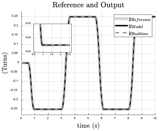
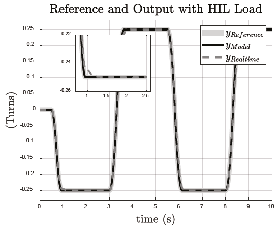
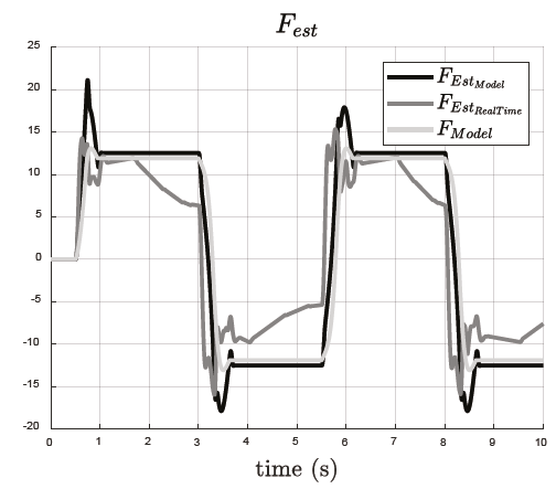
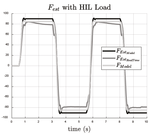
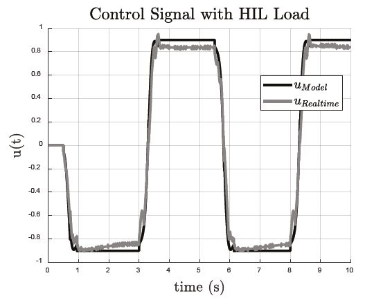
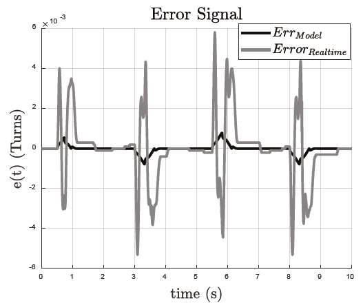
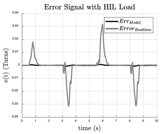
Figure 6 shows the F(t) dynamics for τHIL=0. FModel is function F(t) from model (16). FestModel is the estimation using data obtained from the model (16) using integrals (9) and implemented using FIR filters (10). Estimation FestModel is not equal FModel causing that close-loop dynamics (3) are not zero and condition Festt-Ft0 is not fully met introducing control errors ErrModel as it is shown in Figure 10. FestRealTime is the estimation using real-time data obtained from the servomotors using integrals (9) and implemented using FIR filters (10). FestRealTime further introduces errors (cf. Figure 10) in the control since it has a different behavior than FestModel due noise in the control loop from position and current sensors in the low-level PI current control loop.

Figure 7 shows the Fest dynamics estimation for τHIL 0. In this case it is necessary to notice that HIL load dynamics are about seven times larger as it can be noticed comparing y-axis values of Figure 6 and Figure 7 thus dynamics F(t) in model (19) have a larger contribution of generated load signal (17) due to the fact that τHIL> τint. Estimation behavior is similar introducing difficulties in control errors and close-loop error dynamics. We would expect closer real-time estimation when τHIL0 to the HIL generated dynamics since the nonlinear HIL dynamics are generated with equation (17).

Conclusions

The model-free intelligent control approach has shown its effectiveness in several model and real-time applications considering unknown dynamics employing an estimation integral. The estimation depends on the sampling period for real-time application and the approximation sliding window size that should be small enough so it will not introduce too much delay. Our experimental results show that lose-loop dynamics not zero and condition Festt-Ft0 is not perfectly met introducing control errors; the iPD control strategy is useful if desired control errors are attained. We presented unknown dynamics approximation under demanding test conditions where the controller gain α parameter was not retuned, when using the model-free approach the tuning of parameter α allows to complete the control scheme to attain desired results.

Acknowledgments

The authors would like to thank Prof. Cédric Join from University of Lorraine, Nancy, France, for his useful help for the correct implementation of the estimation integral.

References

Abouaïsa, H., Fliess, M., & Join, C. (2017). On ramp metering: towards a better understanding of ALNIEA via model free control. International Journal of Control, 90(5), 1018-1026. https://doi.org/10.1080/00207179.2016.1193223 [ Links ]

Amasyali, K., Chen, Y., Telsang, B., Olama, M., & Djouadi, S. (2020). Hierarchical model-free transactional control of building loads to support grid services. IEEE Access, 8, 219367-219377. Retrieved on https://doi.org/10.1109/ACCESS.2020.3041180 [ Links ]

Baciu, A., & Lazar, C. (2020). Model-free iPD control design for a complex nonlinear automotive system. On 24th International Conference on System Theory, Control and Computing, 868-873). Retrieved on https://doi.org/10.1109/ICSTCC50638.2020.9259724 [ Links ]

Bara, O., Fliess, M., Join, C., Day, J., & Djouadi, S. (2016). Model-free immune therapy: A control approach to acute inflammation. On 2016 European Control Conference ECC, 2102-2107. Retrieved on https://doi.org/10.1109/ECC.2016.7810602 [ Links ]

Bembli, S., Khraief-Haddad, N., & Belghith, S. (2021). A robust model free terminal sliding mode with gravity compensation control of a 2 DoF exoskeleton-upper limb system. Joournal of Control, Automation and Electrical Systems, 32, 632-641. https://doi.org/10.1007/s40313-021-00687-z [ Links ]

Chekakta, Z., Zerikat, M., Bouzid, Y., & Koubaa, A. (2020). Adaptive fuzzy model-free control for 3d trajectory tracking of quadrotor. International Journal of Mechatronics and Automation, 7(3), 134-146. http://dx.doi.org/10.1504/IJMA.2020.10031292 [ Links ]

Clouatre, M., Thitsa, M., Fliess, M., & Join, C. (2020). A robust but easily implementable remote control for quadrotors: Experimental acrobatic flight tests. On 9th International Conference on Advanced Technologies. Istanbul, Turkey. Retrieved on https://doi.org/10.48550/arXiv.2008.00681 [ Links ]

Doublet, M., Join, C., & Hamelin, F. (2017). Stability analysis for unknown delayed systems controlled by model-free control. On 21st International Conference on System Theory, Control and Computing, 441-446. Retrieved on https://doi.org/10.1109/ICSTCC.2017.8107074 [ Links ]

Elleuch, D. & Damak, T. (2020). Robust model-free control for robot manipulator under actuator dynamics. Mathematical Problems in Engineering. https://doi.org/10.1155/2020/7417314 [ Links ]

Ferrari, M., Park, B, & Olama, M. (2021). Design, evaluation of a model-free frequency control strategy in islanded microgrids with power-hardware-in-the-loop testing. On 2021 IEEE Power & Energy Society Innovative Smart Grid Technologies Conference, 1-5. Retrieved on https://doi.org/10.1109/ISGT49243.2021.9372219 [ Links ]

Fliess, M. & Sira, H. (2003). An algebraic framework for linear identification. ESAIM Control Optimisation and Calculus of Variations, 9, 151-168. [ Links ]

Fliess, M., & Join, C. (2014). Stability margins and model-free control: A first look. On European Control Conference (ECC), 454-459. Retrieved on https://doi.org/10.1109/ECC.2014.6862167 [ Links ]

Fliess, M., & Join, C. (2018). Deux améliorations concurrentes des PID. Automatique, 2(1). https://doi.org/10.21494/ISTE.OP.2018.0284 [ Links ]

Fliess, M., & Join, C. (2021). An alternative to proportional-integral and proportional-integral-derivative regulators: Intelligent proportional-derivative regulators. International Journal of Robust Nonlinear Control, 1-13. https://doi.org/10.1002/rnc.5657 [ Links ]

Fliess, M., Mboup, M., & Sira, H. (2006a). Vers une commande multivariable sans modèle. On Conférence international francophone d’automatique CIFA 2006. Nov., 16-17, Bordeaux, France. Retrieved on https://doi.org/10.48550/arXiv.math/0603155 [ Links ]

Fliess, M., Mboup, M., & Sira, H. (2006b). Complex continuous nonlinear systems: Their back box identification, their control. On 14th IFAC Symposium on System Identification. March 2006, Newcastle, Australia. [ Links ]

Garrido, R., & Soria, A (2005). Estimating the gravity terms in robot manipulators for PD control. International Journal of Robotics & Automation, 20(3), 169-176. http://dx.doi.org/10.2316/Journal.206.2005.3.206-2810 [ Links ]

González-Vargas, A., Serna-Ramirez, J. M., Fory-Aguirre, C., Ojeda-Misses, A., Cardona-Ordoñez, J. M., Tombé-Andrade, J., & Soria-López, A. (2018). A low-cost free-software platform with hard real-time performance for control engineering education. Computer Applications in Engineering Education, 27(2), 406-418. https://doi.org/10.1002/cae.22084 [ Links ]

Han, S., Wang, H., & Tian, Y. (2020). A linear discrete-time extended state observer-based intelligent PD controller for a 12 DOFs lower limb exoskeleton LLE-RePA. Mechanical Systems and Signal Processing, 138, 106547. https://doi.org/10.1016/j.ymssp.106547 [ Links ]

Huba, M., Skrinarova, J., & Bistak, P. (2020). Higher, Order PD and iPD controller tuning. IFAC-PapersOnLine, 53(2), 8808-8813. https://doi.org/10.1016/j.ifacol.2020.12.1388 [ Links ]

Join, C., Abouaïssa, H., & Fliess, M. (2021). Ramp metering: modeling, simulations and control issues. 3rd DECOD Delays and Constraints in Distributed parameter systems. Workshop, Gif-sur-Yvette, France. Retrieved on https://doi.org/10.48550/arXiv.2111.06610 [ Links ]

Join, C., Masse, J., & Fliess, M. (2006). Commande sans modèle pour l'alimentation de moteurs: résultats préliminaires et comparaisons. On Journées Identification et Modélisation Expérimentale JIME 2006. Poitiers, France. [ Links ]

Lafont, F., Balmat, J., Pessel, N., & Fliess, M. (2014). A model-free control strategy for an experimental greenhouse with an application to fault accommodation. Computers and Electronics in Agriculture, 110, 139-149. https://doi.org/10.1016/j.compag.2014.11.008 [ Links ]

Li, X., Wang, Y., Guo, X., Cui, X., Zhang, S., & Li, Y. (2021). An improved model-free current predictive control method for SPMSM Drives. IEEE Access, 9. https://doi.org/10.1109/ACCESS.2021.3115782 [ Links ]

Mboup, M., Join, C., & Fliess, M. (2007). A revised look at numerical differentiation with an application to nonlinear feedback control. On 15th Mediterranean Conference on Control and Automation MED’2007. Athens, Greece. [ Links ]

Mboup, M., Join, C., & Fliess, M. (2009). Numerical differentiation with annihilators in noisy environment. Numerical Algorithms, 50(4), 439-467. https://doi.org/10.1007/s11075-008-9236-1 [ Links ]

Menhour, L., d’Andréa-Novel, B., Fliess, M., Gruyer, D., & Mounier, H. (2018). An efficient model-free setting for longitudinal and lateral vehicle control: validation through the interconnected Pro-SiVIC/RTMaps prototyping platform. IEEE Transactions on Intelligent Transportation Systems, 19(2), 461-475. https://doi.org/10.1109/TITS.2017.2699283 [ Links ]

Qin, Z., Xing, J., & Sun, J. (2020). Dual-loop robust attitude control for an aerodynamic system with unknown dynamic model: Algorithm and experimental validation. IEEE Access, 8, 36582-36594. https://doi.org/10.1109/ACCESS.2020.2974578 [ Links ]

Quanser, C. (2011). (Ver 2.3.603). QuaRC. Markham, Ontario, CA. Retrieved on www.quanser.comLinks ]

Sehili, L., & Boukhezzar, B. (2022). Ultra-local model design based on real-time algebraic and derivative estimators for position control of a dc motor. Journal of Control, Automation and Electrical Systems, 33, 1217-1228. https://doi.org/10.1007/s40313-021-00881-z [ Links ]

Soria, A., Garrido, R, & Concha, A. (2010). Low cost closed loop identification of a DC Motor. On International Conference on Electrical Engineering, Computing Science and Automatic Control, septiembre 8-10. Tuxtla Gutiérrez, México. Retrieved on http://dx.doi.org/10.1109/ICEEE.2010.5608594 [ Links ]

Tebbani, S., Titica, M., Join, C., Fliess, M., & Dumur, D. (2016). Model-based versus model-free control designs for improving microalgae growth in a closed photobioreactor: Some preliminary comparisons. On 2016 24th Mediterranean Conference on Control and Automation (MED), junio 21-24, 683-688. https://doi.org/10.1109/MED.2016.7535870 [ Links ]

The Math Works. (2012). (R2012b). Matlab-Simulink. Natick, MA, USA. Retrieved on www.mathworks.comLinks ]

Villagra, J., d’Andréa-Novel, B., Choi, S., Fliess, M., & Mounier, H. (2009). Robust stop-and-go control strategy: an algebraic approach for nonlinear estimation and control. International Journal of Vehicle Autonomous Systems, 7(3-4). [ Links ]

Wang, H., Xu, H., Tian, Y., & Tang, H. (2020). α-Variable adaptive model free control of iReHave upper-limb exoskeleton. Advances in Engineering Software, 148, 102872. https://doi.org/10.1016/j.advengsoft.2020.102872 [ Links ]

Wang, K., Wang, H., & Tian, Y. (2021). Time-delay estimation based model-free control with adaptive iterative learning compensator for parallel back-support exoskeleton. On IEEE 10th Data Driven Control and Learning Systems Conference, 391, 438-443. https://doi.org/10.1109/DDCLS52934.2021.9455458 [ Links ]

Cómo citar:

Martínez-García, J. C., & Soria-López, A. (2024). Intelligent iPD control estimation of Hardware in-the-Loop generated dynamics. Ingeniería Investigación y Tecnología, 25 (04), 1-9. https://doi.org/10.22201/fi.25940732e.2024.25.4.031

Received: December 26, 2022; Accepted: September 18, 2024

Creative Commons License This is an open-access article distributed under the terms of the Creative Commons Attribution License