1 Introduction

Triangular and hexagonal tilings of the plane have received attention for several decades for 2D digital image modeling, as alternative to the tiling of square tiles which may be identified with the set of pixels or grid points in the discrete plane (cℤ)2 (c∈ℝ, c>0). Triangular pixels have been used, for example, to study convexity properties of digital objects [¹³], to develop geometrical transformations [¹], to design digital topological spaces and thinning algorithms [³, ⁷, ¹⁰, ¹¹], and for data visualization [⁹]. The present article considers binary digital images defined on triangular tilings, where the pixels are identified with triangular tiles being all congruent each other. The digital objects of interest are represented as connected sets of tiles, using edge- and vertex-adjacency based connectivity types.

Boundary tracing, also called contour tracing or contour following, is a standard digital image processing segmentation method which determines the frontier of an object. Well-known boundary tracing algorithms for 4- and 8-connected objects in (cℤ)2 are described, for example, in the widely used textbooks [⁴, ⁵, ⁸], they can be equally used for sets of square tiles modelled by 4- or 8-adjacency graphs. Boundary tracing was generalized for edge-adjacency-connected subsets of rectangular tilings in [¹⁷].

The previous conference paper [¹⁸] presented an algorithm of boundary tracing for edge-adjacency-connected subsets of the tiling of equilateral triangles, equivalently for sets of triangular pixels. The resulting so-called canonical boundary path was used in [¹⁸] to determine the minimal perimeter polygon (MPP) for objects whose boundaries are digital Jordan curves. In [¹⁶], the properties of the canonical boundary path were further studied and exploited in an MPP algorithm for more general digital objects, which are certain edge-adjacency-connected sets of triangular tiles called regular complexes.

The present article continues studying boundaries in triangular tilings, it proposes a boundary tracing algorithm for connected digital objects of triangular tiles or pixels, permitting both edge-adjacency and vertex-adjacency based connectivity types. The algorithm is illustrated by examples and compared with previously known algorithms for triangular pixels. The resulting boundary sets and paths are studied under both connectivity types, where it arises as necessary to distinguish between boundaries and contours.

In the remaining, Section 2 introduces connectivity, objects and boundaries in triangular tilings. Section 3 presents the boundary tracing algorithm, Section 4 studies properties of boundaries and contours. The proposed algorithm is compared to two algorithms previously known from the literature. Some conclusions complete the paper.

2 Connectivity, Digital Objects and Boundaries in Triangular Tilings

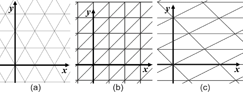
By a triangular tiling T we mean a family of congruent non-degenerated triangles named tiles, whose union covers the plane, and where the intersection of any two tiles, either is empty, or is a common side of both tiles, called an edge of the tiling, or is a point which is a common vertex of six tiles. Hence T is an edge-to-edge polygonal tiling of the plane due to [⁶]. Let the tiling be positioned as shown in Figure 1, where the tiles form rows parallel to the x-axis. This can always be achieved since the union of any two triangular tiles which share an edge, forms a parallelogram. The tiles of T are of two types which occur alternating in each row. In the standard triangular tiling, see Figure 1(a), the triangles are equilateral, and each row has alternating upright and inverted triangles.

Fig. 1 Examples of triangular tilings, positioned as aligned to the Cartesian coordinate system, (a) shows the standard case of the tiling of equilateral triangles 

Two distinct tiles of T which intersect each other, share a side, or, share a vertex. For each T∈T, there are three other tiles sharing a side with T, and twelve tiles T′≠T which intersect T by sharing at least a vertex. Similarly to the well-known 4- and 8-adjacencies for square pixels, this gives rise to the following two adjacency relations on the set T:

Definition 1 Let T1, T2 be distinct tiles of a triangular tiling T .

– T1, T2 are called edge- adjacent or 3-adjacent or 3-neighbors if they share a common side.

– T1, T2 are called vertex- adjacent or 12-adjacent or 12-neighbors if they intersect each other, that is, they have a common vertex.

For k∈{3, 12}, if T1, T2 are k-neighbors, we say that T1 is a k-neighbor of T2.

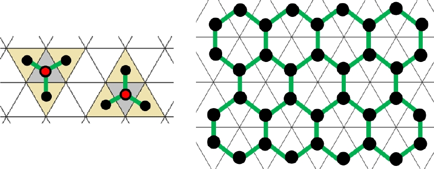
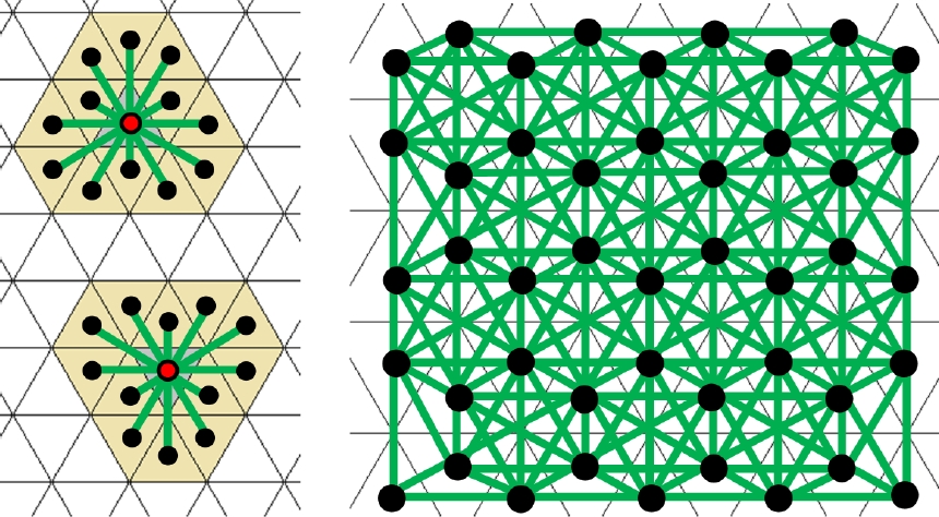
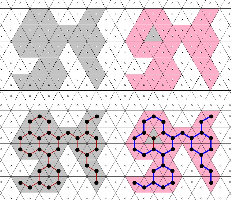
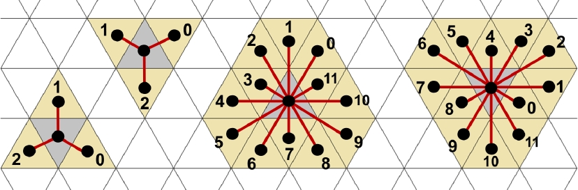
The k-adjacency, k∈{3, 12}, is a non-reflexive symmetric binary relation on T. 3-neighbors also are 12-neighbors, but generally not vice versa. The k-adjacency generates a graph G(T) called k-adjacency graph with node set T, its edges are given by the pairs of k-neighbors, see Figures 2 and 3 where each tile is presented by its centre point drawn as a black dot, and the graph edges are depicted as green straight line segments. These centre points form a discrete set in the plane which is distinct from ℤ2 but could be the support (i.e., the set of pixels) of a digital image. The 3-adjacency graph is planar, which means that it can be presented in ℝ2 drawing its nodes as points and its edges by line or curve segments such that these intersect each other only in points that represent nodes. The 12-adjacency graph is not planar since it cannot be presented in such a way.

Fig. 2 3-neighbors and a portion of the 3-adjacency graph for the standard triangular tiling 

Fig. 3 12-neighbors and a portion of the 12-adjacency graph for the standard triangular tiling 

Graph theory provides paths and connectivity: a k-path is a sequence of tiles (T1, T2, ⋯, Tn) such that Ti is a k-neighbor of Ti+1, i∈{1, ⋯, n−1}. It is called a closed k-path if also Tk is a k-neighbor of T1. A set A⊂T is k-connected if any two tiles of A are connected via a k-path in A. If A has at least two tiles, T∈A is an end tile if T is k-adjacent to exactly one other tile of A.

For any set of tiles C⊂T and k∈{3, 12}, a subset A⊂C is called a k-component of C if it is a maximal k-connected subset of C, that is, A is k-connected, and for any tile T∈C\A, A∪{T} is not k-connected. Clearly, if C is k-connected, C coincides with its unique k-component.

Recall that the tiles of a triangular tiling are of two types. Note that all 3-neighbors of a triangular tile of a given type are tiles of the other type, hence the tiles in any 3-path alternately are of both types. In particular, a 3-path in the standard triangular tiling has alternately upright and inverted triangles.

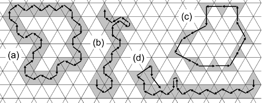
Analogous to the well-known simple curves in the 4- and 8-neighborhood graphs of ℤ2 [⁸], a simple k-path or Jordan k-curve is a closed k-path whose each element has exactly two k-neighbors in this path, see Figure 4.

Fig. 4 In the standard triangular tiling, (a) shows a Jordan 3-curve, (b) a non-simple 3-path, (c) a Jordan 12-curve and (d) a non-simple 12-path 

For any set of tiles C⊂T, let us denote its point set union by |C|=∪C ={p∈ℝ2:p∈T for a tile T∈C}⊂ℝ2. We define a (digital) object as any finite non-empty subset C of T.

Definition 2 (from [12, 13]) Let T be a triangular tiling and C⊂T an object. The set of tiles of C that intersects the topological frontier fr(|C|), is called the boundary ℬ(C) of C. Any closed k-path, for k∈{3, 12}, that consists of all tiles of ℬ(C), is named a boundary k-path of C.

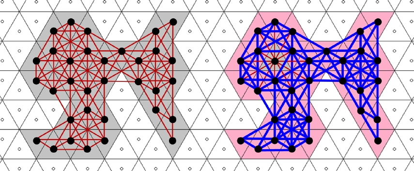
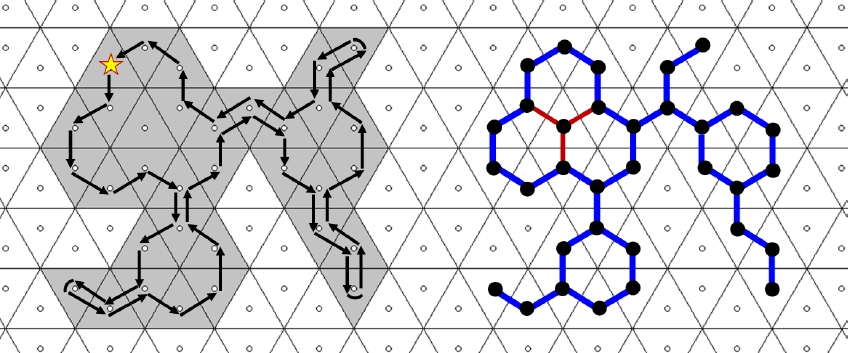
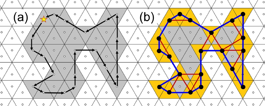
Whereas ℬ(C) is a uniquely defined set, C may have several boundary k-paths with distinct properties. If ℬ(C) is not k-connected then C has no boundary k-path at all. Figure 5 presents a 3-connected object with its boundary due to Definition 2. This object has several boundary 3-paths and 12-paths but none of them is simple since the object (as well as its boundary) has end tiles. Under the 3-connectivity, the object also has thin parts where any boundary 3-path must pass twice. Since any 3-connected object also is 12-connected, it can be considered as a subgraph of the 12-adjacency graph as shown in Figure 6.

Fig. 5 A 3-connected object (shaded grey) with its boundary highlighted in pink. The subgraph induced by the object in the 3-adjacency graph is shown presenting its tiles as black dots (being the graph nodes), the object graph edges as brown lines, and the graph edges between boundary tiles as thick blue lines 

Fig. 6 The object from Figure 5 and its boundary are shown as induced subgraphs of the 12-adjacency graph, the object graph edges are drawn as brown lines, the graph edges between boundary tiles as bold blue lines 

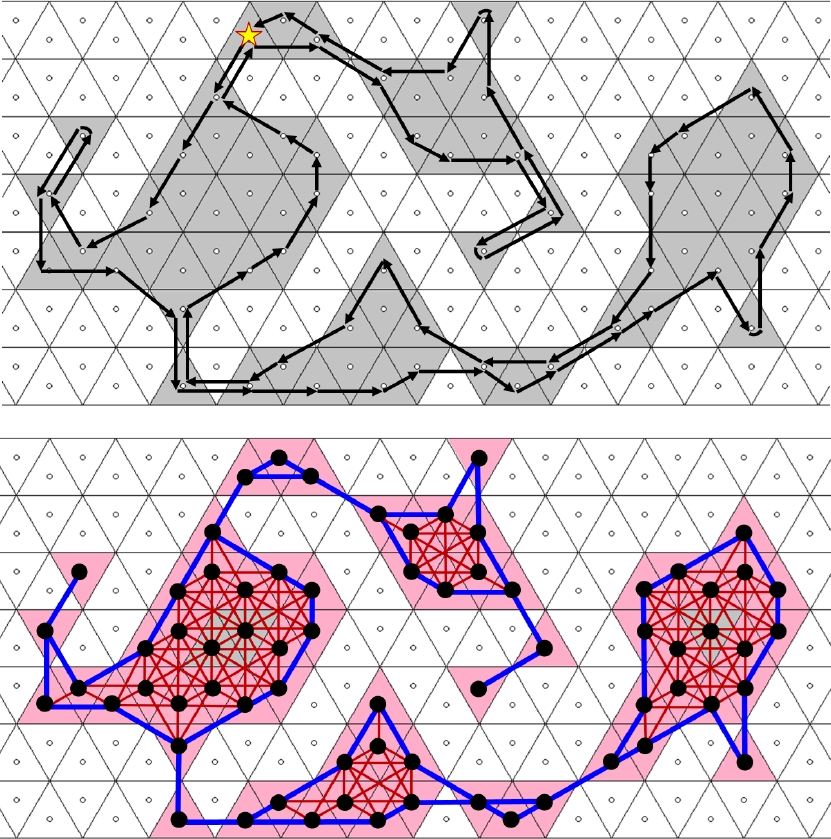
Figures 7 and 8 show a 12-connected object with its boundary, also presented as a subgraph of the 12-adjacency graph. This object is not 3-connected, it has thirteen 3-components.

Fig. 7 A 12-connected object (shaded grey) with its boundary tiles highlighted in pink 

Fig. 8 The object from Figure 7 is presented as induced subgraph of the 12-adjacency graph 

3 Boundary Tracing and Contours for 3- and 12-Connected Objects

The previous articles [¹⁶, ¹⁸] proposed a boundary tracing algorithm for 3-connected objects in the standard triangular tiling.

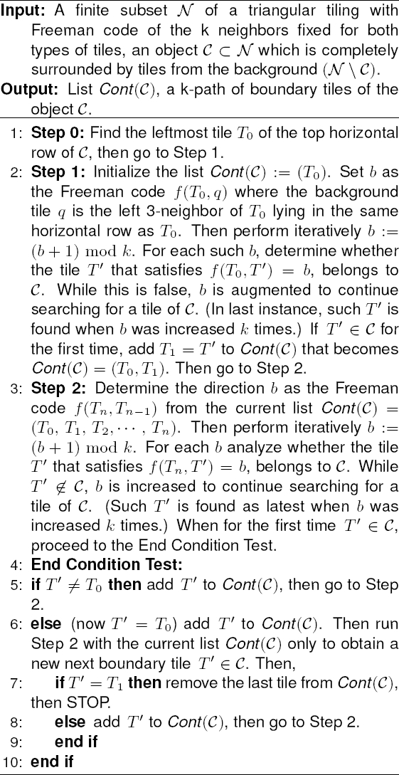
The more general Algorithm 1 presented in this section is suitable for any k-connected object C with k∈{3, 12} in a triangular tiling T, supposing that C has at least two tiles and |C|⊂ℝ2 has no hole. We also assume that there exists a finite set N with C⊂N⊂T such that the background tiles from (N\C) fully surround the object C.

Algorithm 1 Boundary tracing for a k-connected object C in a triangular tiling, where C has at least two tiles, and |C|⊂ℝ2 has no hole. 

Similar as known for adjacency graphs for square pixels, for any tile T∈G(N), we employ the Freeman code to represent the movement direction from T to each of its k-neighbors T′, which is coded by a number f(T, T′)∈{0, 1, 2, ⋯, k−1}. As result, any k-path in G(N) may be described by its Freeman chain code, see Figure 9.

Fig. 9 Freeman codes for 3-neighbors and 12-neighbors in the standard triangular tiling 

In the standard triangular tiling, a 3-path has alternately upright and inverted triangles. This is not in general true for a 12-path which uses more possible movements. So, a 3-path can be reconstructed from its Freeman chain code whenever the type of the starting tile is known. For reconstructing a 12-path, it would be necessary to store also the types of tiles, together with the Freeman codes.

Boundary tracing starts with finding a first boundary tile. This can be achieved, for example, by detecting the leftmost tile T0 of the top row of C, as included in Algorithm 1, by scanning N on horizontal rows from the left to the right. Clearly then T0∈ℬ(C), and T0 has a left 3-neighbor q in the same horizontal row (independently of the connectivity type of C), where q belongs to the background. In particular, using the Freeman code as in Figure 9 for the standard triangular tiling, if T0 is an upright triangle and f(T0, q)=1, or, if T0 is an inverted triangle and f(T0, q)=2, then q∉C.

For each last boundary tile Tn found, Algorithm 1 determines the Freeman code b=f(Tn,Tn−1), that is, of the direction from Tn back to Tn−1. Then it inspects the tile T′ which lies in direction (b+1) mod⁡ k, if T′ belongs to C then it is the next boundary tile found. Otherwise, the tile T′ lying in direction (b+2) mod⁡ k is inspected, it is the next boundary tile if it lies in C. If not, the process is continued, inspecting the tiles T′ in directions (b+3) mod⁡ k, (b+4) mod⁡ k, ⋯, (b+(k−1)) mod⁡ k, until for the first time, T′ is found to belong to C. If all these inspected tiles T′ are in the background, then the tile in direction (b+k) mod⁡ k belongs to C and is the next boundary tile. The last case only occurs if Tn is an end tile of C, we have then Tn+1=Tn−1.

Algorithm 1 determines a uniquely defined k-path Cont(C)=(T0, T1, T2, ⋯, Tn) such that, when boundary tracing would be continued, the next tiles found would be, again, Tn+1=T0, Tn+2=T1. Step 2 will found T0 again, when boundary tracing is finished, but this may occur also if Cont(C) touches itself at T0 but continues differently, the End Condition Test distinguishes between both situations. Since the Freeman codes from Figure 9 generate counterclockwise orders of the k-neigbors, the resulting k-path goes through the boundary in counterclockwise sense.

For the standard triangular tiling and k=3, with Freeman codes fixed as in Figure 9, Step 1 of Algorithm 1 must set b:=1 if T0 is an upright triangle, and b:=2 if T0 is an inverted triangle.

In the previous works [¹⁶, ¹⁸] where exclusively 3-connected objects were considered, the resulting 3-path of Algorithm 1 was called canonical boundary path of C. We will see in Section 4 that for 12-connectivity, it is necessary to distinguish between a boundary k-path due to Definition 2 and the list constructed by Algorithm 1. This justifies the following definition.

Definition 3 Let C⊂T be a k-connected object, k∈(3, 12) in a triangular tiling T, such that C has at least two tiles and |C|⊂ℝ2 has no hole. Any k-path b=(T0, T1, ⋯, Tn) of tiles of C which, up to appropriate shifting of the cyclic sequence b, coincides with the sequence Cont(C) determined by the Boundary Tracing Algorithm (Algorithm 1), is called the k-contour of C.

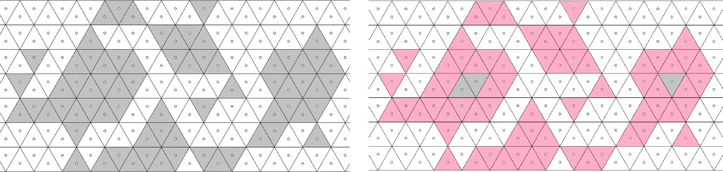
Figure 10 presents the 3-contour obtained by Algorithm 1 of a 3-connected object, comparison with Figure 5 reveals that the set of tiles belonging to the 3-contour coincides with the boundary due to Definition 2, the 3-contour is a boundary 3-path. The situation is distinct for the 12-connected object shown in Figure 11, where not all boundary tiles participate in the 12-contour.

Fig. 10 The 3-contour of the object from Figure 5 is illustrated by black arrows, it starts at the leftmost tile of the top row which is marked by a star in the figure, its Freeman chain code begins as (2, 2, 2, 0, 0, 0, 2, 2, 2, 2, 1, 0, 0, 0, 0, 1, ⋯). The path has alternating upright and inverted triangles. The right figure shows the 3-contour as induced 3-adjacency subgraph, each tile is presented by its centre point, the graph edges between boundary tiles are drawn bold in blue and the other object graph edges as brown lines 

Fig. 11 The 12-contour of the object from Figure 7 is illustrated by black arrows. Figure below: the graph edges between tiles belonging to the 12-contour Cont(C) are drawn as thick blue lines, the other object graph edges as brown lines. In the underlying tiling, the boundary tiles are highlighted in pink 

Algorithm 1 has linear time complexity depen-ding on the number of boundary tiles that belong to the k-contour, k∈{3, 12}. Step 0 needs constant time to find T0, and Step 1 performs at most k tests to determine T1. For each last found tile Tn, Step 2 uses at most k tests to determine Tn+1. Note that Algorithm 1 does not inspect all object tiles if the object is distinct from its boundary.

4 Boundaries and Contours

By the construction performed by Algorithm 1, any k-contour is a closed k-path which lies within the boundary due to Definition 2. For 3-connected objects, Algorithm 1 coincides with the boundary tracing algorithm from [¹⁶, ¹⁸] where only 3-connectivity was considered and the resulting 3-path was called the canonical boundary path of C. This is justified by the following property.

Lemma 1 Let C be a 3-connected object with at least two tiles and such that |C| has no hole, in a triangular tiling. Then the following is true:

(1) The boundary ℬ(C) is 3-connected.

(2) The 3-contour Cont(C) is a boundary 3-path.

(3) ℬ(C) coincides with the set of tiles that belong to Cont(C).

(4) Any boundary 3-path that traces the boundary counterclockwise, that is, which corresponds to visit fr(|C|) counterclockwise, coincides with Cont(C) or a shifted version of Cont(C).

Proof: Let C be a 3-connected object satisfying the hypothesis. Then the boundary ℬ(C)⊂C has at least two tiles. By the hypothesis, fr(|C|) is a Jordan curve¹ which is touched from its interior by any boundary tile T, where T∩fr(|C|) is a side or a vertex of T.

(1) The curve fr(|C|) is made of sides of triangles which are boundary tiles. Let T1, T2 tiles in ℬ(C) that intersect only in a vertex v (then T1, T2 are not edge-neighbors). Assume that s1 is a side of T1 and s2 a side of T2 such that {v}=T1∩T2=s1∩s2 and s1∪s2 belongs to fr(|C|), then v∈fr(|C|). Since C is 3-connected, there exists a tile T3∈C with vertex v, hence T3∈ℬ(C) and T3 is a 3-neighbor of T1 and of T2. In consequence, ℬ(C) is 3-connected.

(2) Algorithm 1 follows the curve fr(|C|) without interruption to include into Cont(C) all tiles of C that intersect fr(|C|), no matter whether this intersection is a triangle side or a vertex. As result, all tiles of ℬ(C) are contained in Cont(C), hence Cont(C) is a boundary 3-path.

(3) By the construction made by Algorithm 1, Cont(C) is a closed 3-path that lies in ℬ(C). By the previous part (2), ℬ(C) is contained in the set of tiles belonging to Cont(C). Hence ℬ(C) is equal to the set of tiles contained in Cont(C).

(4) Let B=(T1, T2, ⋯, Tn) be any (closed) boundary 3-path that traces the boundary ℬ(C) in counterclockwise sense. Then, when traveling through the sequence B, each tile Ti visited touches fr(|C|) such that at the “right side” of Ti, the intersection ai=Ti∩fr(|C|) is a vertex or a side of Ti, with the result that a1∪a2∪ ⋯ ∪an reproduces the curve fr(|C|) in counterclockwise sense. This implies that for any Ti∈B, the next tile Ti+1∈B (computing i+1 and i−1 modulo n) is the first object tile which can be found when inspecting the 3-neighbors of Ti in counterclockwise order. This coincides with the procedure of Algorithm 1 to find each next tile of the 3-contour. Since T0∈ℬ(C), it appears in B. But T0 also belongs to Cont(C). As a consequence, the cyclic sequence B coincides with Cont(C) up to an appropriate shifting.

The following characterization of 3-contours is useful because it uses neither Algorithm 1 nor the curve fr(|C|).

Lemma 2 Let C be a 3-connected object with at least two tiles and such that |C| has no hole, in a triangular tiling T, and T∈C. Then T belongs to the 3-contour Cont(C) if and only if T has a 12-neighbor Q∈(T\C).

Proof: T∈ Cont(C)⊂ℬ(C) implies that T has a common point with fr(|C|) which is a vertex of T, hence T has a 12-neighbor Q∈(T\C). On the other hand, if T∈C has a 12-neighbor Q∈(T\C) then T intersects fr(|C|, hence T∈ℬ(C). By Lemma 1 and since fr(|C| is a Jordan curve, there exists a boundary 3-path that traces the boundary counterclockwise and contains T, hence this 3-path coincides with Cont(C) which consequently contains T.

Applying Lemma 2, it is easy to find a tile T0 belonging to the 3-contour of a 3-connected object C with at least two tiles and such that |C| has no hole. Then if q∉C is a 3-neighbor of T0, a modified version of Algorithm 1 can start with these tiles T0 and q to construct the 3-contour.

Although the boundary of a 12-connected object is 12-connected, similar properties as those in Lemma 1 do not hold in general for 12-connected objects. Figure 12 shows the 12-contour of the 3-connected object from Figure 10. Recall also Figure 11 where the tiles belonging to the 12-contour form a proper subset of the boundary. These examples confirm that for 12-connected objects the boundary may not coincide with the set of tiles belonging to the 12-contour, hence the 12-contour is not a boundary 12-path, and not every boundary 12-path counterclockwise tracing the boundary coincides with the 12-contour.

Fig. 12 The 3-connected object from Figure 10 also is 12-connected, hence Algorithm 1 can determine its 12-contour which is illustrated in (a) by black arrows. (b) shows the 12-contour as induced subgraph of the 12-adjacency graph, the tiles participating in the 12-contour are filled yellow, the graph edges corresponding to pairs in the 12-contour are drawn as bold blue lines, other graph edges between tiles belonging to the 12-contour are depicted as brown lines 

5 Comparison with Previous Boundary Tracing Algorithms

Besides our papers [¹⁶, ¹⁸] where a boundary tracing algorithm for 3-connected objects was proposed, it seems that only two works from the literature consider boundary tracing in relation to sets of triangular tiles. The first one from [¹³] uses boundary tracing as preprocessing for an algorithm to determine the minimal perimeter polygon (MPP) of so-called normal complexes, which corresponds to vertex-connected objects without end tiles, in certain polygonal tilings. The second work, published in [¹⁴, ¹⁵] and briefly summarized in [⁸], develops oriented adjacency graphs to model discrete sets and presents a generic contour tracing algorithm.

Both cited works do not explicitly treat boundary tracing for objects in triangular tilings, but the abstract structures developed there include that case. It turns out that the boundary tracing algorithm from [¹³] is erroneous, and that our Algorithm 1 is a specified and completed version of the “Border Mesh Determination” from [¹⁵].

5.1 Boundary Tracing in Polygonal Tilings

The articles [¹², ¹³] are considered pioneering works on the development of the minimal perimeter polygon (MPP) and its application to study convexity properties of digital objects whose elements are identified with the tiles of polygonal tilings of the plane. Whereas rectangular tilings are used in [¹²], theoretical foundations are developed in [¹³] where the pixels are modelled by convex polygons belonging to a tiling P where for any two tiles T1, T2 that intersect each other, T1∩T2 is a full side or a vertex of both polygons and T1∪T2 forms a convex polygon. In [¹³], a non-empty finite set C⊂P is called a normal complex if it has no end tile and |C| is simply connected in ℝ2. For a normal complex C⊂P, the existence of a unique MPP of C is proved and an algorithm to determine the MPP is presented in [¹³].

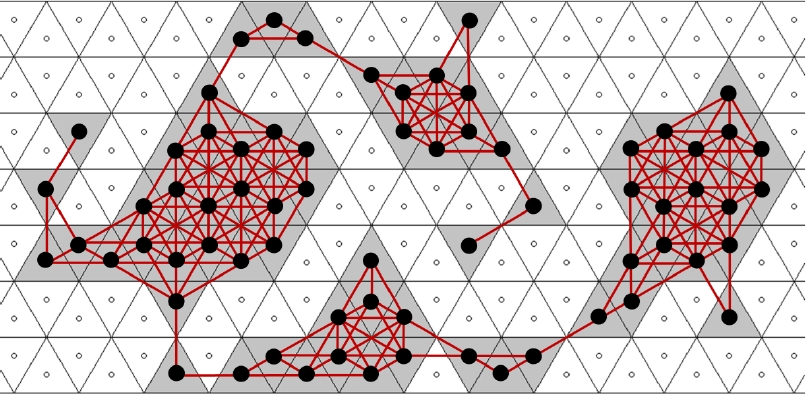
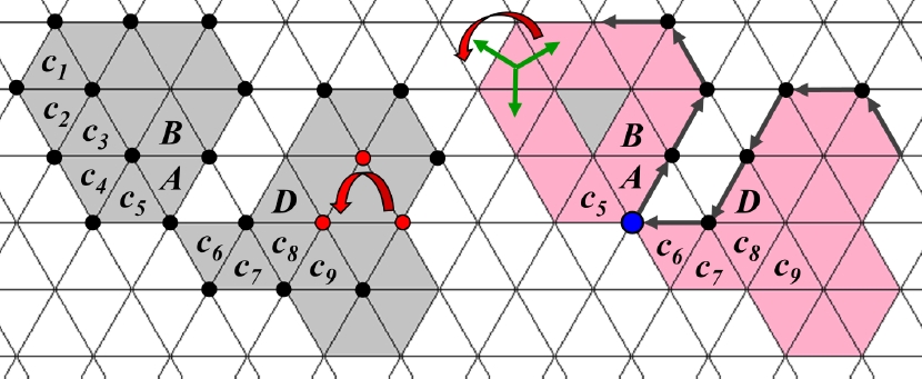
The assumptions in [¹³] are satisfied for any triangular tiling T. In our terminology, a normal complex C⊂T is a 12-connected object without end tile where |C| has no hole. If T1, T2∈C such that T1∩T2={v} for a common vertex v of both tiles, v is called a cut point for C in [¹³]. Any 12-connected object which is not 3-connected, has a cut point, such as the object in Figure 13.

Fig. 13 A 12-connected object (shaded grey) in a triangular tiling which illustrates the performance of the boundary tracing algorithm from [¹³]. The boundary is highlighted in pink in the right figure. The algorithm pretends to find the sequence (c1, c2, c3, c4, c5, c6, c7, ⋯) of boundary tiles. See the text for explanations 

The MPP algorithm in [¹³] needs as preprocessing step the determination of a boundary 12-path due to Definition 2. For example, for the object in Figure 13, the “Algorithm M” in Section “MPP algorithm” of [¹³] aims first to construct the sequence (c1, c2, c3, c4, c5, c6, c7, ⋯) of boundary tiles, this order corresponds to visit the curve fr(|C|) in counterclockwise sense.

How to find this path of boundary tiles of an object C, is only detailed in the Appendix “An illustrative implementation of Algorithm M” of [¹³] as follows: a data structure is constructed that contains for each tile T whether it belongs to C or not. The vertices of the convex polygon T are counterclockwise ordered and for each pair (vi, vi+1) of consecutive vertices of T, a pointer is established to the “bordering tile” T′, that is, where T∩T′=(vi, vi+1)¯ is a common side. This creates an order of pointers from T to all tiles that have a common side with T. Boundary tracing starts at a boundary tile c1∈C that has a side belonging to fr(|C|), and the pointer from c1 to some tile S∉C. Then the subsequent pointers from c1 are used to inspect the addressed tiles until finding a first object tile which is taken as c2. For each last found boundary tile ck, the pointer from ck to ck−1 is considered and the next pointer from ck starts to inspect the addressed tiles, until finding a first object tile which is taken as ck+1. The process stops when ck+1=c1, then the boundary sequence is affirmed in [¹³] to have been completed.

In a triangular tiling, by the definition of the pointers in [¹³] an object is considered under 3-connectivity, and the boundary tracing determines the boundary 3-path of any 3-connected object in the same manner as our Algorithm 1, but no ending situation treatment is performed in [¹³]. More importantly, consider the 12-connected object C in Figure 13 which is not 3-connected. The boundary tracing of [¹³] correctly determines the first boundary tiles c1, c2, c3, c4, c5. Then the pointer from c5 back to c4 is considered, the next pointer from c5 indicates a background tile, but the next pointer addresses the object tile denoted as A in Figure 13. Restarting from A, the tile B results as the next boundary tile found. The cut point c5∩c6 (drawn as blue dot in Figure 13) is ignored and c6 cannot be found as the next boundary tile. So, the algorithm from [¹³] is erroneous for 12-connected objects that are not 3-connected.

6 Conclusion and Future Work

This paper presents a boundary tracing algorithm (Algorithm 1) for objects in triangular tilings modelled for k∈{3, 12} as oriented k-adjacency graphs. For the special case k=3, Algorithm 1 coincides with the preliminary version from [¹⁶, ¹⁸] which is applied there within another algorithm to find the minimal perimeter polygon (MPP) of certain type of objects. The MPP has been successfully applied, for example in [¹², ¹³], to study convexity properties of such objects.

To develop our Algorithm 1, the “Border Mesh Determination” algorithm from [⁸, ¹⁴, ¹⁵] was com-pleted and adapted to the oriented k-adjacency graphs (k∈{3, 12}) of triangular tilings.

This article also proves some properties of boundaries and k-contours of objects of triangular tiles which can be applied in future works for object description and recognition.

Future research includes to continue to study properties of 12-contours for 12-connected objects in triangular tilings, to consider other adjacencies, and to analyze digital Jordan curves and their topological separation properties. Another aim is to look for applications of k-contours in digital image analysis and pattern recognition, where modeling objects as sets of triangular tiles results as useful, for example, for the triangular covers from [²].

References

1. Avkan, A., Nagy, B., Saadetoglu, M. (2020). Digitized rotations of 12 neighbors on the triangular grid. Annals of Mathematics and Artificial Intelligence, Vol. 88, pp. 833–857.
[ Links ]
2. Biswas, A. et al. (2018). Triangular covers of a digital object. Journal of Applied Mathematics and Computation, Vol. 58, pp. 667–691. DOI: 10.1007/s12190-017-1162-8.
3. Deutsch, E. (1972). Thinning algorithms on rectangular, hexagonal, and triangular arrays. Communications of the ACM, Vol. 15(9), pp. 827–837.
4. Gonzalez, R., Woods, R. (2018). Digital Image Processing (Global Edition). Pearson Education Limited, USA, 4rd edition.
5. Gonzalez, R., Woods, R., Eddins, S. (2020). Digital Image Processing using Matlab. Gatesmark Publishing LLC, USA, 3rd edition.
6. Grünbaum, B., Shephard, G. (1978). Tilings and Patterns. W.H. Freeman and Company, USA.
7. Kardos, P., Palágyi, K. (2015). Topology preservation on the triangular grid. Annals of Mathematics and Artificial Intelligence, Vol. 75, pp. 53–68. DOI: 10.1007/s10472-014-9426-6.
8. Klette, R., Rosenfeld, A. (2004). Digital Geometry - Geometric Methods for Digital Picture Analysis. Morgan Kaufmann Publisher, USA.
9. Nagy, B. (2022). Diagrams on the hexagonal and on the triangular grids. Acta Polytechnica Hungarica, Vol. 19(4), pp. 27–42.
10. Nagy, B. (2024). A Khalimsky-like topology on the triangular grid. In Brunetti, S., et al., editors, Proc. of DGMM 2024. Springer, LNCS 14605, Switzerland, pp. 150–162. DOI: 10.1007/978-3-031-57793-212.
11. Saha, P., Rosenfeld, A. (2001). Local and global topology preservation on locally finite sets of tiles. Information Sciences, Vol. 137, pp. 303–311. DOI: doi:10.1016/S0020-0255(01)00107-4.
12. Sklansky, J., Chazin, R., Hansen, B. (1972). Minimum perimeter polygons of digitized silhouettes. IEEE Trans. on Computers, Vol. 21(3), pp. 260–268. DOI: 10.1109/TC.1972.5008948.
13. Sklansky, J., Kibler, D. (1976). A theory of nonuniformly digitized binary pictures. IEEE Trans. on Systems, Man, and Cybernetics, Vol. 6(9), pp. 637–647. DOI: 10.1109/TSMC.1976.4309569.
14. Voss, K. (1988). Theoretische Grundlagen der digitalen Bildverarbeitung. Akademie-Verlag Berlin, German Democratic Republic.
15. Voss, K. (1993). Discrete Images, Objects, and Functions in Zn. Springer, Serie Algorithms and Combinatorics Vol.11, USA.
16. Wiederhold, P. (2024). Computing the minimal perimeter polygon for digital objects in the triangular tiling. Discrete Applied Mathematics, Vol. (under review), pp. 1–33.
17. Wiederhold, P. (2024). Computing the minimal perimeter polygon for sets of rectangular tiles based on visibility cones. Journal of Mathematical Imaging and Vision, Vol. 66, pp. 873–903. DOI: 10.1007/s10851-024-01203-z.
18. Wiederhold, P. (2024). On the minimal perimeter polygon for digital objects in the triangular tiling. In Mezura-Montes, E., et al., editors, MCPR 2024 Mexican Conf. on Pattern Recognition. Springer, LNCS Vol. 14755, Switzerland, pp. 141–154. DOI: 10.1007/978-3-031-62836-814.
nueva página del texto (beta)
Inglés (pdf)
Artículo en XML
Referencias del artículo
Enviar artículo por email
Citado por SciELO