


 nueva página del texto (beta)
 Inglés (pdf)
 Artículo en XML
 Referencias del artículo
 Enviar artículo por email
 Citado por SciELO
  Similares en
SciELO
Similares en
SciELO 
 Permalink
1. Introduction
Mineral precipitation poses a significant challenge in the production pipelines of geothermal wells (Mercado et al., 1989). This issue primarily hinges on the chemical composition of the brine as well as the well's pressure, temperature, and mass flow conditions. Hydrogeochemical modeling serves as a valuable tool for replicating or predicting natural and technologically induced processes, including corrosion, scale formation, degassing, and more (White et al., 2000; Lichti et al., 2005; Bozau et al., 2015). The presented predictive model aims to estimate the time required for the formation of incrustations primarily composed of minerals, specifically amorphous silica, within a pipeline. This estimation serves as one of the input data points for calculating the filling percentage. It is assumed that most of the minerals responsible for scaling originate from a brine film covering the pipe, and the volume of this film represents a proportion of the water volume circulating within the pipe during the fluid's residence time. This volume proportion is referred to as the parameter "k".
Dissolved silica in the brine primarily consists of silicic acid monomers. The precipitation of monomeric silica and subsequent particle formation leading to scale formation can be attributed to fluctuations in temperature and pH levels. In certain instances, these scales can disrupt the brine circulation, which serves as a heat transfer medium. Scale formation can hinder the process of brine re-injection into the reservoir and, in severe cases, compel the shutdown of power plants due to significant scaling. As noted by Durham and Walton (1999), removing scale in geothermal power plants is often a formidable challenge that can result in equipment damage over prolonged periods of operation. Consequently, this can result in an overall increase in the plant's operational expenses.
This study investigates the accumulation of amorphous silica within the Los Humeros Geothermal Field (LHGF) wells, which has been in a liquid state since the inception of depositing in the production area. Substantial reductions in temperature and pressure at these wells have led to the formation of thick crusts, particularly prevalent at shallower depths, where they rapidly evaporate (Guiza 1977; Ocampo-Díaz et al., 2005). To correlate the parameters, field data from several wells of LHGF (H-01, H-13, H-15, H-16, H-17, H-17D, H-19, H24, H-32, and H-33) is used. The operating conditions and depth where fouling occurs are obtained from observational field data (Cornejo, 1996; Torres, 1995; Quijano and Torres, 1995). This data serves to simulate the behaviour of wells through equations of up-flow and heat as described in this work. The pressure and temperature conditions that determine precipitation are obtained from the results of these simulations. While the moles of the majority of minerals that precipitate per kilogramme of water are determined using speciation codes and thermodynamic precipitation (Pérez et al., 2012) in conjunction with algorithms that describe the kinetic precipitation of silica in an aqueous solution (Gimón-Bastidas et al., 2018).
2. Previous work
In the LHGF, various studies have been reported in the literature regarding the petrological characterization, thermal conditions, and alteration conditions in certain wells. For instance, Viggiano Guerra and Robles Camacho (1988a) and b), Viggiano Guerra (1988), Prol-Ledesma and Browne (1989a, 1989b), and Martínez-Serrano and Alibert (1994), Prol-Ledesma (1998), Martínez-Serrano (2005), González-Partida et al. (1991a), González-Partida et al. (1992a), González-Partida et al. (1992b), González-Partida et al. (1993a, 1993b), González-Partida et al. (2022), Viggiano-Guerra et al. (2013), Izquierda-Montalvo et al. (2014), and Pandarinath et al. (2023) have all contributed to this body of knowledge. Similarly, several works have explored radiogenic isotopic and fluid geochemistry aspects, as documented by Arnold and González-Partida (1986a, 1986b, 1987), Barragán et al. (1989), Barragán et al. (1991), González-Partida et al. (1991b), Cedillo-Rodríguez (1999), and Izquierdo-Montalvo et al. (2000). González-Partida et al. (2001), Barragán et al. (2002), and Yáñez-Dávila (2018) have also highlighted the high concentrations of silica in both brine and hydrothermal mineralogy.
Silicic alteration assemblages primarily consist of quartz and quartz polymorphs such as cristobalite and opal. These assemblages are typically found beneath or in proximity to sinters. Additionally, silica polymorphs tend to precipitate in the discharge pipes of hydrothermal fluids as they pass through turbines. The presence of high proportions of quartz within deep alteration assemblages (as depicted in Figure 1 and 2) signifies the distribution of deep, high-temperature argillic alteration assemblages. Truesdell (1991), Bienkowski et al. (2003), and Bienkowski et al. (2005) have previously documented the connection between deep, high-silica alterations and acidic fluids in the LHGF.
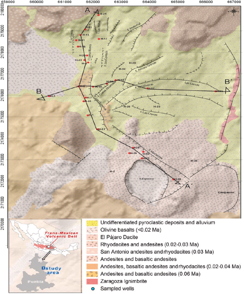
Figure 1 Local geology of the Los Humeros Geothermal Field (Puebla, central-south Mexico), showing the locations of two geological sections (A-A' and B-B') displayed in Figure 2 and the wells sampled in this study. Modified from González-Partida et al. 2022.
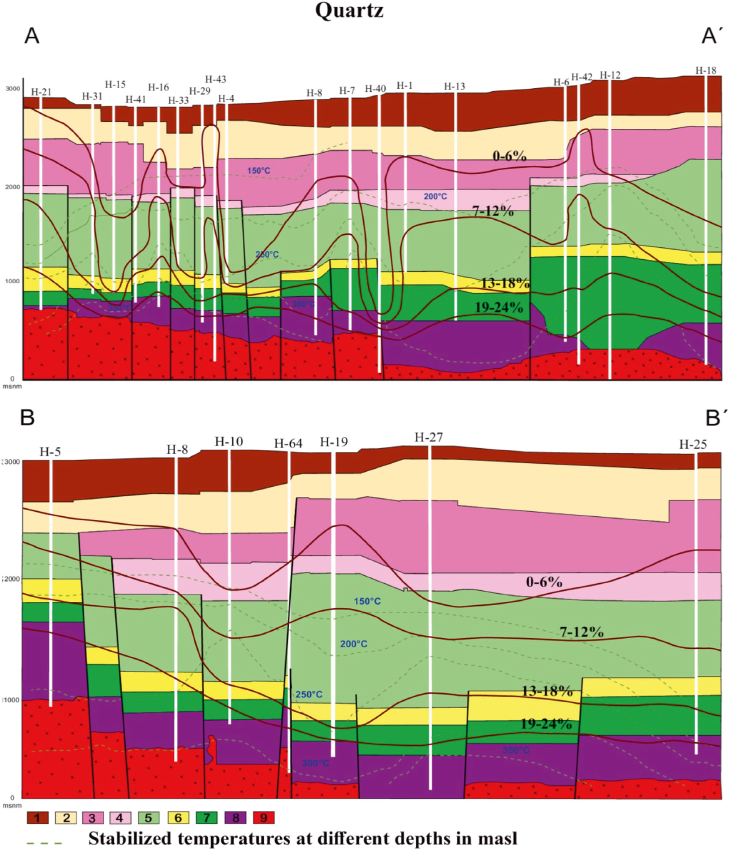
Figure 2 Los Humeros Geothermal Field sections A-A' and B-B': Distribution of quartz (in %), compared with stabilized temperatures obtained from well measurements (in °C = dashed lines). Modified from González-Partida et al. 2022. Key: 1 = pumice, basalts, and andesites; 2 = lithic tuffs; 3 = ignimbrites; 4 = vitreous tuffs and ignimbrites; 5 = augite andesites; 6 = vitreous tuffs; 7 = hornblende andesites; 8 = limestones and skarn; 9 = granodiorites.
Similarly, several studies have explored the abundance of silica in relation to deep acidic supercritical fluids, often characterized by high concentrations of HCl, HF, and B in well fluids (Prol- Ledesma, 1998; Tello, 1992; Tello et al., 2000; Bernard et al., 2013). A notable characteristic of the LHGF is the high fraction of water vapor in brines with pH levels between 1 and 3 in deep, high-enthalpy wells (Arellano et al., 2003; Izquierdo-Montalvo et al., 2014). Acidic fluids in this context may result from various factors, including the exsolution of vapor from a relatively shallow hypabyssal intrusive body, deep high-temperature degassing of supercritical fluids, changes in temperature or pressure, boiling in the geothermal environment (shallow low-temperature boiling of subcritical fluids), reactivation of fractures, or oxygen leakage. Truesdell (1991) and D'Amore and Panichi (1980) have postulated the origin of these acids in the LHGF, possibly emanating from an unknown source like a magma chamber beneath the geothermal system, releasing acids such as HCl and HF into aquifers.
2.1. LOS HUMEROS GEOTHERMAL FIELD (LHGF)
LHGF is situated in Puebla, at the eastern end of the Mexican volcanic belt (19° 40' north latitude; 97° 25' west longitude), approximately 200 km from Mexico City, at an elevation of 3000 meters above sea level (as shown in Figure 1). LHGF marks the northern boundary of the Serdán-Oriental basin (Figure 1). This region is renowned for its bimodal, monogenetic volcanism, characterized by small, isolated cinder and scoria cones, large rhyolitic domes, and both rhyolitic and basaltic maars.
Exploratory studies in LHGF commenced in 1962, initiated by the Federal Electricity Commission (Mena and González, 1978; Perez, 1978; Yáñez et al., 1979; Palacios and Garcia, 1981). The first well was drilled in 1982, and electricity production began in 1990 with the commissioning of the first 5 MW generators. Subsequently, more than 40 wells have been drilled, and by 1995, there were seven units, each with a capacity of 5 MW (Quijano and Torres, 1995). Presently, the field has an installed capacity of 40 MW (Gutiérrez-Negrin, 2007).
Since the early stages of exploration and production, numerous geochemical and engineering studies have been conducted on deposits in their natural state, confirming the presence of two deposits (Arellano et al., 1998). The shallower deposit, located between 1600 and 1025 meters above sea level (MASL), is characterized by a liquid phase at temperatures ranging from 300°C to 330°C and a neutral pH. In contrast, the deeper deposit, situated below 850 MASL, exhibits convective behavior, with steam typically rising from the reservoir and condensing into fluid. This deposit has a low liquid saturation and operates at temperatures between 300 °C and 400 °C (Barragán et al., 2008). LHGF, with the exception of well H-01, has a high enthalpy of production, and the fluid is predominantly vapour. Heat transfer dominates the fluids in the wells, which in some cases are fed from the shallowest deposit, sometimes from the deepest, and sometimes from both (Torres, 1995).
Wells such as H-01, H-13, H-15, H-16, H-17, H-19, H-33, and H-24 (Figure 2), among others, experienced reduced production due to mineral precipitation and corrosion. In some instances, extended downtime was necessary for repairs (Cornejo, 1996; Gutiérrez and Viggiano, 1990).
The calculation of flow within wells requires the consideration of momentum transport, which includes inertia and viscous forces between fluids and between fluids and the well walls. Flows within wells are characterized by high speeds, often turbulent behavior, significant pressure gradients, and phase changes. Therefore, the calculation of flow within wells must primarily yield realistic values for density, pressure, and temperature as functions of the position along the drilling shaft. The mathematical foundations for this computational development are outlined below.
3.Methodology
3.1. ANALYTICAL APPROACH AND CALCULATIONS
In the present study, we employ the equations of mass, momentum, and energy conservation to characterize the flow within wells. There exist correlation-based and flow regime-based models that have proven effective in describing this type of flow, obviating the need for separate simulations of two- phase dynamics. We utilize a non-linear system of first-order differential equations, originally developed by Gimon-Bastidas et al. (2018) and integrate it with the algorithms in our study. This system simulates the kinetic dissolution and precipitation of minerals in aqueous electrolyte solutions, and it is applicable across a temperature range of 20 °C to 320 °C, pressures from 1 to 1000 bar, and ionic strengths of up to 6 mol/kg (Gimon-Bastidas et al., 2018). Their numerical tool provides accurate estimations of the following: a) the types and concentrations of minerals dissolved or precipitated over time; b) the ions and cations generated and released during the kinetic dissolution or precipitation of one or more minerals in the solution (Gimon-Bastidas, et al. 2018).
In this article, we simulate the wells using a direct modeling approach based on the work of Gimon-Bastidas et al. (2018). We establish the conditions of pressure, temperature, enthalpy, and specific volume at the depth where amorphous silica filling occurs.
3.1.1. DETERMINATION OF THE TIME AT WHICH AN AMORPHOUS SILICA RING ADHERES TO THE INNER WALLS OF THE PIPELINES
As amorphous silica constitutes the predominant hydrothermal mineral phase at LHGF, silica is employed to model the incrustation processes. The precipitation of amorphous silica is most frequently encountered in pipe seals (Ocampo-Díaz et al., 2005; Miranda-Herrera, 2012), and the literature extensively documents that the sealing of pipes with amorphous silica (Cornejo, 1996; Gutiérrez and Viggiano, 1990) is the primary issue facing the geothermal industry (see Figure 3). Over time, the accumulation of amorphous silica in pipelines and fluid handling equipment proves detrimental to geothermal power production. The observations made in LHGF are included in Appendix A, providing ample observational data for adjusting and validating the proposed model. Studies conducted at the Hellisheidi geothermal power plant in SW-Iceland on solution composition, saturation indices, and silica precipitations have indicated silica precipitation rates exceeding 0.35-0.75 g m-2 day-1 (Van den Heuvel et al., 2018). The determination of the time required for amorphous silica scale formation relies on the following assumptions: 1) The mass flow within the pipe section remains constant; 2) The temperature, pressure, and enthalpy within this section remain consistent; 3) The pipe maintains a uniform diameter; 4) In LHGF, the predominant phase undergoing precipitation is amorphous silica; 5) Scale formation occurs regularly and uniformly; 6) Kinetically precipitated amorphous silica originates from a film whose volume represents a percentage of the water flowing through the pipe; 7) The brine is in equilibrium before entering the pipe section, but after entering, the fluid's temperature decreases, leading to precipitation.
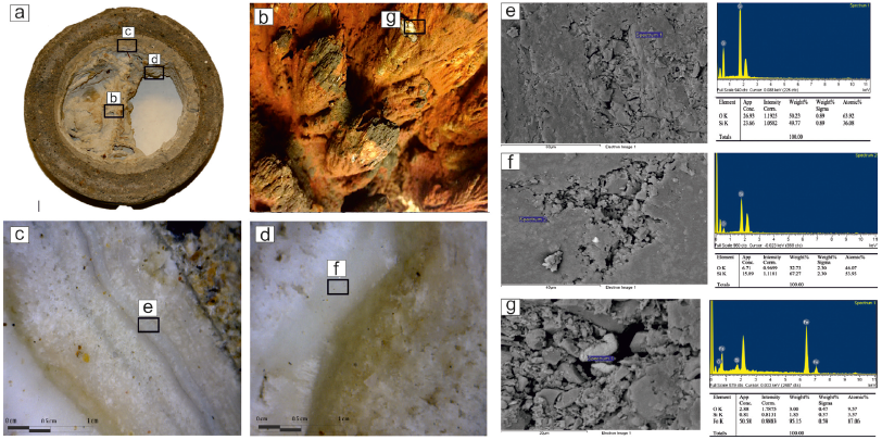
Figure 3 (a) Sealed pipe of the H-43 well at a depth of 2500 m, where the precipitation of amorphous silica can be observed (c and d), and amorphous silica with a hematite patina (b). Note the banded texture of progressive growth toward the center of the pipe. Boxes e, f, and g correspond to the areas where SEM-EDS analyses were performed, shown in microphotographs. SEM-EDS analyses reveal the compositions of the components: amorphous silica in e) and f); hematite in g) from the red patina (b).
3.1.2. DETERMINATION OF TOTAL MOLES OF AMORPHOUS SILICA DEPOSITED PER KILOGRAM OF WATER
Brines found in geothermal wells contain a large amount of dissolved ionized salts, primarily chlorides and sulfates, which are highly corrosive (Valdez et al., 2009). The chemical analysis of the brine extracted from the Humeros wells is presented in Table 1 (Arellano et al., 2001). The pH of the various brines varies, ranging from acidic (pH 5) to basic (pH 8.9), depending on the location of the well and changes over time. In the case of well H-16 brine, with a pH of 5.1, reports of corrosion exist despite having samples with a neutral pH (Gutiérrez and Viggiano, 1990). These solutions were used to determine the moles of kinetically deposited amorphous silica per kilogram of water
Table 1 Concentration of species in electrolytic aqueous solutions used in this work.
| Ions in Electrolyte solution (Esp.) |
H-01 | H-15 | H-16a | H-16b | H-16c | H-17 | H-19 | H-20 | H-30 | H-31 | H-32 | H-33 |
|---|---|---|---|---|---|---|---|---|---|---|---|---|
| Cl- | 180 | 10 | 268 | 265 | 99 | 159 | 1479 | 349 | 408 | 14 | 330 | 180 |
| HCO3- | 33 | 10 | 1x10⁻⁶ | 144 | 464 | 42 | 3 | 1.3 | 260 | 26 | 9.5 | 33 |
| SiO2 | 911 | 502 | 363 | 651 | 551 | 519 | 970 | 727 | 152 | 970 | 915 | 911 |
| SO4-2 | 55.7 | 132 | 37 | 191 | 142 | 75 | 106 | 21 | 14 | 0.6 | 16 | 55.7 |
| Na+ | 180 | 120 | 43 | 494 | 586 | 112 | 340 | 122 | 112 | 112 | 107 | 180 |
| K+ | 27 | 15 | 9 | 26 | 32 | 19 | 45 | 19 | 14 | 14 | 21 | 27 |
| Li+ | 0.4 | 0.47 | 0.02 | 1.1 | 0.85 | 0.4 | 1.1 | 0.41 | 0.23 | 0.42 | 0.24 | 0.4 |
| Ca+2 | 1.7 | 1.2 | 3 | 2.8 | 0.9 | 0.84 | 4.5 | 23 | 0.8 | 1 | 5.3 | 1.7 |
| Mg+2 | 0.04 | 0.07 | 0.02 | 0.09 | 0.05 | 0.03 | 0.4 | 0.05 | 0.08 | 0.08 | 0.18 | 0.04 |
| pH | 7.7 | 5.2 | 5.1 | 7.7 | 8.9 | 7.6 | 5 | 6.8 | 5.3 | 7.7 | 5.7 | 7.7 |
Table 2 Amount of mineral per kg of water, in moles
| Minerals | H-01 | H-15 | H-16 | H-17 | H-19 | H-20 | H-30 | H-31 | H-32 | H-33 |
|---|---|---|---|---|---|---|---|---|---|---|
| Quartz (SiO2(aq)) | 147.97 | 89.35 | 77.78 | 147.07 | 59.48 | 11.90 | 56.62 | 84.26 | 60.67 | 50.55 |
| Calcite(CaCO3) | 89.10 | 78.16 | 67.44 | 39.85 | 0.00 | 0.00 | 58.45 | 0.00 | 0.00 | 0.00 |
It can take thousands of years for the interactions between brine and rock to reach a state of equilibrium with the surrounding minerals, such as potassium chloride, sodium chloride, etc., or saturation with certain salts like silica, bicarbonate, sulfide, and sulfate (Mercado et al., 1989). Pérez et al., (2012) utilized the temperatures listed in Table 3 and the thermodynamic equilibrium code SPCALC to determine the state of equilibrium between the brine (Table 1) and the rock (Table 2). After calculating the concentrations of species at equilibrium and the amount of thermodynamically precipitated amorphous silica, the kinetic precipitation of the amorphous silica phase was measured at a temperature 5 °C lower than the equilibrium temperature. Following the determination of kinetically precipitated moles at each of the evaluated temperatures, correlations corresponding to each well were established (Table 3).
Table 3 Correlations for the calculation of kinetically deposited moles of amorphous silica.
| Well | T (oC) | Correlation with respect to time t (s) |
|---|---|---|
| H-01 | 280 |
|
| H-13 | 283 |
|
| H-15 | 304 |
|
| H-16 | 305 |
|
| H-17 | 275 |
|
| H-19 | 275 |
|
| H-20 | 270 |
|
| H-24 | 289 |
|
| H-32 | 281 |
|
| H-33 | 284 |
|
3.1.3. KINETIC PARAMETER CALCULATION
To determine the moles of kinetically precipitated amorphous silica
Appendix B provides the equation defining the reaction rate for this system. The pressures used in both thermodynamic speciation and kinetic precipitation correspond to vapor pressure. Results from kinetic precipitation are presented in Figure 4 through 8 (5, 6, 7).
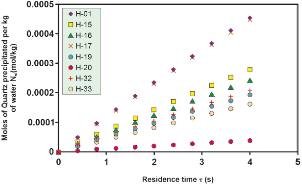
Figure 4 Kinetic precipitation of amorphous silica at a temperature of 290o C for the different wells studied.
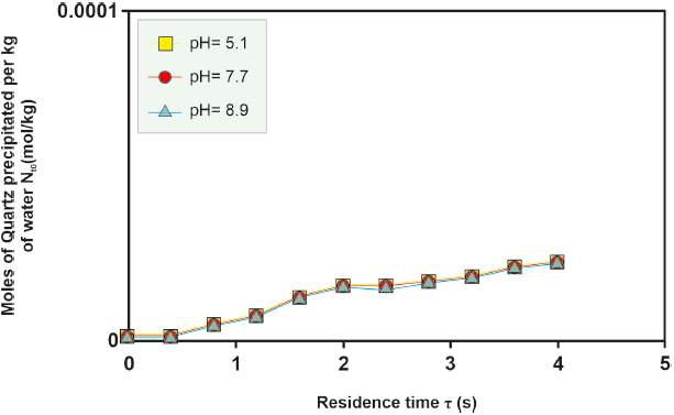
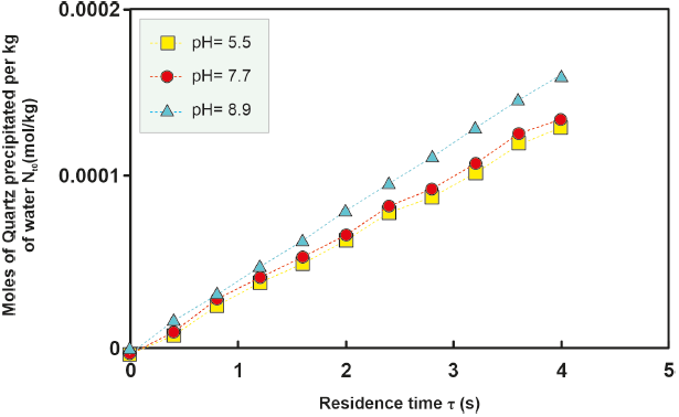
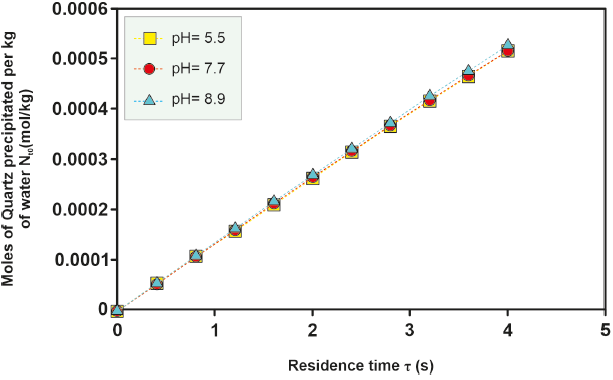
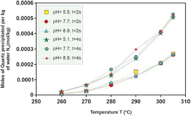
Figure 8 Kinetic precipitation of amorphous silica at different temperatures over a time of 2s and 4s for well H-16.
The kinetics of amorphous silica precipitation for the various wells under study exhibit consistent behavior with increasing temperature. As temperature rises, the quantity of kinetically precipitated amorphous silica also increases. This trend is evident in Figure 4, where the ordinate axis is an order of magnitude greater than that in Figure 5.
For the H-16 well, an investigation into the effect of pH on the moles of kinetically precipitated amorphous silica was conducted. Differences in the moles of amorphous silica precipitated in solutions with varying pH levels increase at temperatures between 280 °C and 300 °C and decrease at lower (260 °O280 °C) and higher (> 300 °C) temperatures, as depicted in Figure 4, 5, 6, 7, 8. However, the sealing time for the H-16 well was determined based on the solution with a pH of 5.1, as this solution best represents the behavior of the well during the study period (Arellano et al., 2001; Cornejo, 1996; Gutierrez and Viggiano, 1990).
The algorithm summarizing the methodology used to determine the value is depicted in Figure 9. For each of the wells, a correlation was established between the moles of kinetically precipitated amorphous silica and the variables of time and temperature at the sealing point (Table 3).
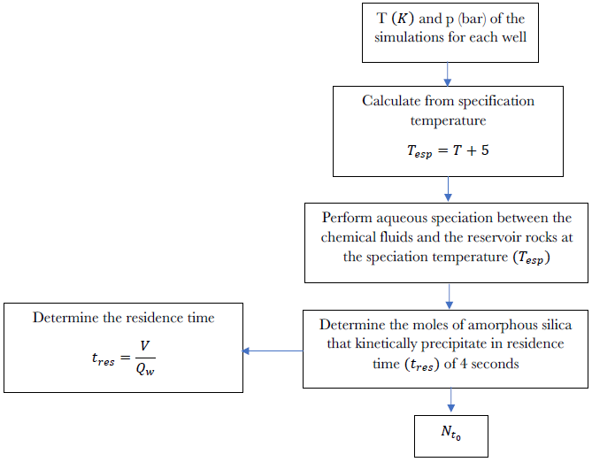
Figure 9 Algorithm used in the determination of kinetically precipitated moles of amorphous silica per kg of water. Aqueous speciation was performed for each of the chemical fluids of the wells studied in a temperature range of 260o C to 300o C.
Another parameter required for input into the
Where, VW is the volume of water entering the pipe section under study in the first iteration and QW is the flow of water.
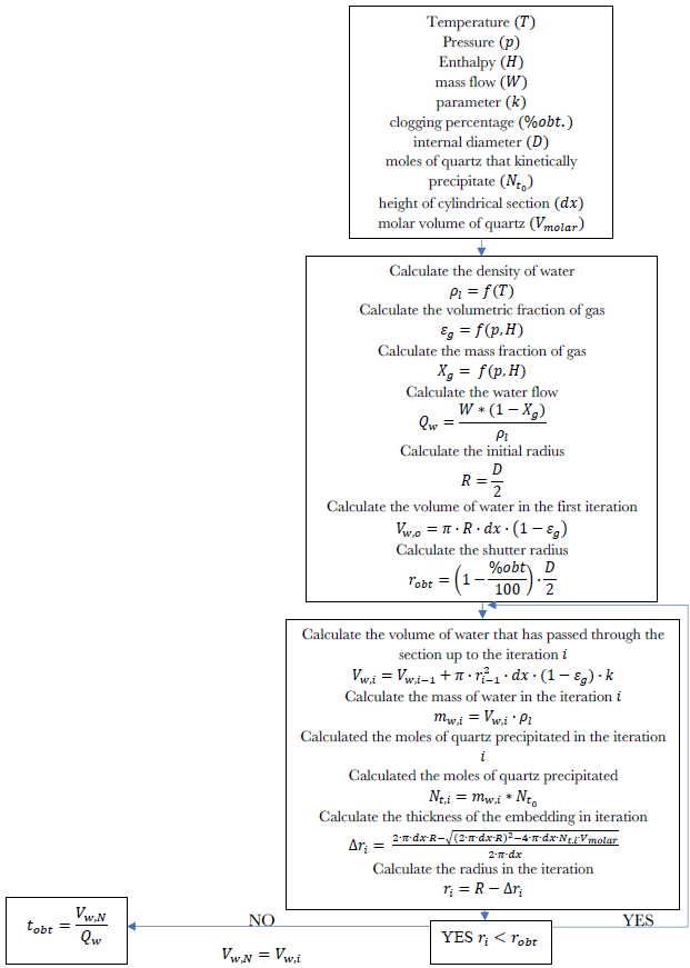
3.5. DETERMINING THE TIME AT WHICH THE AMORPHOUS SILICA RING FORMS
The two main assumptions regarding the shape of the scale and the origin of the kinetically precipitated amorphous silica are as follows: 1) The scale forms as a uniform cylindrical ring and adheres to the inner wall of the pipe (see Figure 3); 2)The amorphous silica that precipitates kinetically originates from a water film, the volume of which corresponds to a percentage of the total water present in the cylindrical section at the residence time of the water body; 3) This percentage of volume is known as the ‘k’ parameter and is an adjustable parameter.
In determining the time when the amorphous silica ring forms, the following input variables are utilized: a) Pressure conditions (p), temperature (T), enthalpy (H), and mass flow rate (W) in the section of the pipe under investigation. The first three conditions are obtained from well simulations, while the mass flow rate is reported by Cornejo (1996), Quijano and Torres (1995), Torres (1995), and the Institute of Electrical Research; b) The percentage of pipe clogging (%Obt), which is either derived from literature data (Gutiérrez and Viggiano, 1990) or determined based on increased pressure in the well; c) The percentage of the total volume that constitutes the water film (k). This parameter is adjustable; d) The internal radius of the pipe (R); e) Moles of kinetically deposited amorphous silica per kilogram of water
The radius obtained after ring formation (Equation 3) remains constant throughout the calculation of the ring formation time or shutter time:
Every time the cylindrical section is filled with liquid an iteration occurs. (i), at each iteration (i) The resulting radius is calculated (ri) after the kinetic precipitation of amorphous silica using Equation 4. The algorithm for calculating training time of the amorphous silica ring, stops when:
The variation of the internal radius of the pipe (
Where, dx is the height of the cylindrical section, which is calculated as dx = L/nx. L is the total length of the pipe and nx is the number of subdivisions.
Moles of amorphous silica deposited
Where
Where
Where
Where N is the total number of iterations, Knowing that,
The time elapsed until the given shutter radius is reached
4. Thermodynamic simulation of the wells used in the adjustment of the predictive model
Cornejo (1996) and Gutiérrez and Viggiano (1990) have provided data pertaining to the formation of amorphous silica scale in wells H-01, H-13, H-15, H-16, H-17, H-19, H-24, and H-33, all located in the LHGF in Mexico. These authors offer comprehensive information regarding the performance and operational conditions of these wells. This information encompasses values such as the enthalpy of production (Hcab), mass flow rate of the mixture (W), depth (L), pipe diameter (D), bottom temperatures (Tf), wellhead temperatures (Tcab), the location of the scale within the well, the commencement date of production, and the date of scale occurrence or well repair.
Table 4 presents a summary of the field data employed for simulating the pressure and temperature profiles of the wells used in adjusting and validating the predictive model shown in Figure 11. This table illustrates that the temperature profiles were simulated using the mathematical model of flow and heat.
Table 4 Input data used in well simulation.
| Well | D (m) | W (kg/s) | L (m) | Tf (oC) | Tcab (oC) | pcab (bar) | Hcab (kJ/kg) |
|---|---|---|---|---|---|---|---|
| H-01 | 0.17a | 48a | 1450a | 280b | 239.86c | 31d | 1190d |
| H-13 | 0.17a | 6.94a | 2414a | 315d | 203.08c | 15d | 1622d |
| H-15 | 0.17a | 16.94a | 1970a | 320d | 257.80c | 39d | 2456d |
| H-16 | 0.17a | 20a | 2048a | 318d | 248.40c | 38d | 2661d |
| H-17 | 0.17a | 12.5a | 2265a | 300b | 218.14c | 22a | 2660d |
| H-17Df | 0.24a | 5.5f | 1695f | 315e | 236.49c | 22e | 2664e |
| H-19 | 0.17a | 12.5a | 2292a | 290 | 229.20c | 22d | 2640d |
| H-20 | 0.17a | 10.88f | 2252f | 270e | 249.87c | 35d | 2435d |
| H-24 | 0.21a | 5.5a | 3280a | 300 | 235.82c | 27a | 2490c |
| H-32 | 0.24f | 9.72f | 1699f | 307e | 222.47c | 25d | 1997d |
| H-33 | 0.17a | 10a | 1600a | 298e | 242.24c | 34d | 2594d |
a) Cornejo 1996; b) Quijano and Torres 1995; c) Calculated with the mathematical simulator; d) Torres 1995; e) Supplied by IEE (Electrical Research Institutes); f) Well H-17D is a well deviated from the horizontal in its repair (Cornejo 1996)
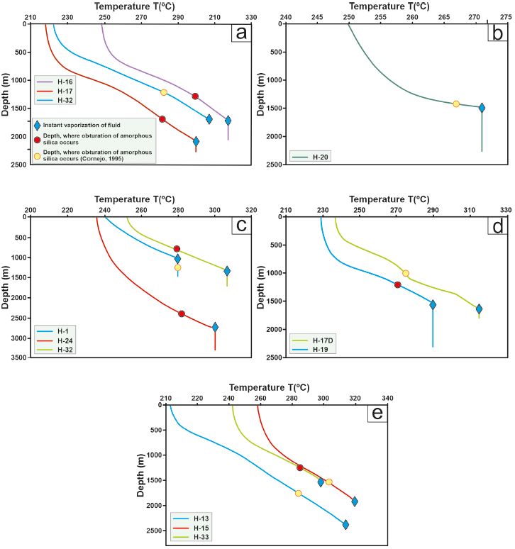
Figure 11 Temperature profiles of the LHGF studied versus the depth at which the seal is located in each of the wells. (a) Wells H-16, H-17, and H-32. (b) Well H-20. (c) Wells H-01, H-24 and H-32. (d) Wells H-17D and H-19. (e) Wells H-13, H-15, and H-33.
4.1. MODEL ADJUSTMENT PREDICTING AMORPHOUS SILICA SCALE FORMATION TIME
The parameter ‘k’ was adjusted using results obtained from simulations of six wells: H-01, H-13, H-15, H-16, H-17, and H-19. The H-01 well commenced production in 1982 (Cornejo 1996) and remained productive until 1994. In 1995, maintenance was performed on the pipe, and a seal was discovered between depths of 1295 m and 1450 m in its productive zone (Cornejo, 1996). Notably, this is the only well where the sealing zone aligns with initial conditions where the fluid was entirely in the liquid phase (see Figure 11(c)). In contrast, Wells H-13, H-15, H-16, H-17, H-17D, H-19, H-20, H-24, H-32, and H-33 had seals at shallower depths, occurring before instantaneous vaporization of the fluid and resulting in significant temperature and pressure losses within the formation or grid (refer to Figure 11). The Los Humeros reservoir conditions, which have governed the productive behavior since its inception, are as follows: fluids within the region of subcooled liquid near the saturation curve, low permeability, and low porosity of the system. A decrease in pressure leads to a phase change within the rock formation. Los Humeros is characterized by a low-porosity system that allows for efficient heat transfer from the rock to the fluid. Consequently, there are enthalpy variations between the wellhead and the well bottom on the order of 1200 kJ/kg. Additionally, the low permeability results in high pressure gradients between the well bottom and the wellhead (Quijano and Torres, 1995).
Thermodynamic simulations provide a close approximation to the reported values of wellhead pressure and enthalpy (Torres, 1995; Cornejo, 1996), with errors of less than 15%. Notably, Wells H-01 and H-15 (see Figure 12(b)), which draw from a single reservoir (Torres, 1995), exhibit differences in behavior. H-01, characterized by low temperatures and minimal pressure loss, experiences limited heat transfer between the fluid and the surrounding medium. Consequently, the enthalpy difference between the wellhead and the bottom is very similar, with a difference of merely 40 kJ/kg lower at the wellhead compared to the bottom. This well exhibits the highest fraction of liquid among those studied in the Humeros region.
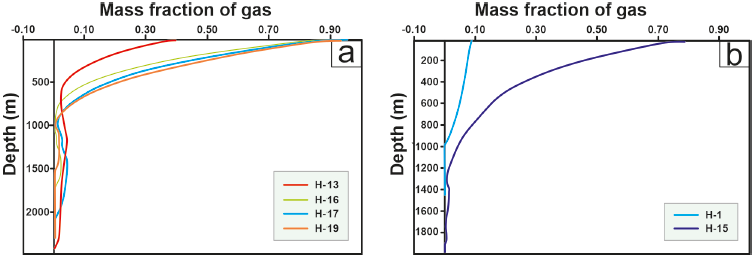
Figure 12 Gas fraction profiles of the wells in the LHGF. (a) Wells fed from two reservoirs. (b) Wells fed by a single reservoir.
On the other hand, H-15, being the deepest well and closest to the central collapse, has higher bottom temperatures, significant contact with low-porosity rock after instantaneous vaporization, and a considerable temperature difference with the surrounding rock, favoring additional heat transfer. This results in a significantly higher fraction of steam and, consequently, a greater enthalpy difference between the wellhead and the bottom (Quijano and Torres, 1995), on the order of 1100 kJ/kg.
The enthalpy behavior and vapor fraction of Wells H-13, H-16, H-17, and H-19 (see Figure 12(a)) align with the hypothesis that these wells draw from two reservoirs (Arellano et al., 1998; Torres, 1995). Vapor fraction plots reveal that the deepest reservoir, characterized by higher temperatures, experiences early boiling and high permeability, leading to a substantial pressure loss on the order of 90 bar (Quijano and Torres, 1995). This reservoir does not exhibit vapor gain beyond the instantaneous vaporization point, with vapor fractions remaining below 0.05 (see Figure 12(a) and Figure 13(c)). However, when the well is also fed by the shallower deposit, vapor gain occurs at heights near the wellhead. This behavior is not typical of dry wells with biphasic fluids since their formation (Arellano et al., 2011), as observed in H-20 and H-24, which draw from a single reservoir.
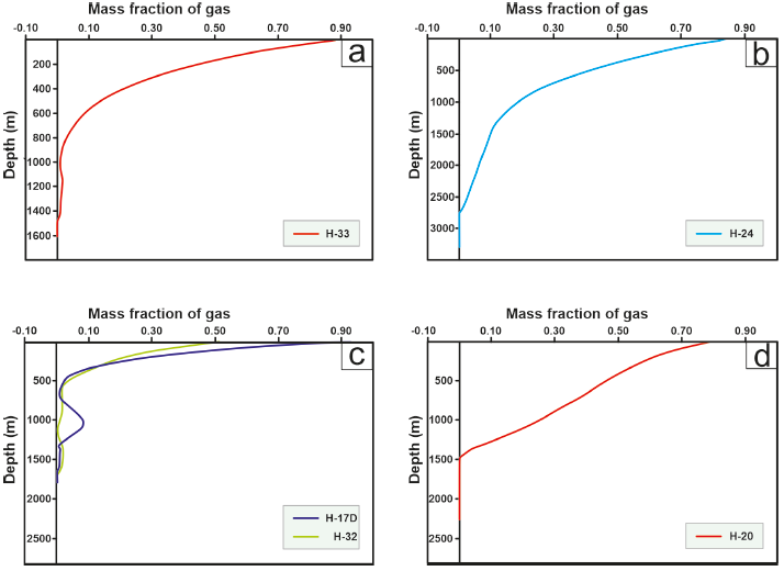
Figure 13 Profiles of the gas mass fraction of the wells in the LHGF. (a) Well H-33, fed by two reservoirs, used for model adjustment. (b) Well H-24, fed by a reservoir, used for model adjustment. (c) Wells H-17D and H-32, fed by two reservoirs, used to estimate operating time. (d) Well H-20, fed by a reservoir, used to estimate operating time.
The results obtained by simulating wells drawing from one or two reservoirs indicate that the algorithms developed in this study can also replicate the behavior of these wells. This expands the applicability of the mathematical model of flow and heat due to the diversity of well types in the LHGF. Another phenomenon observed aligns with Ocampo-Díaz et al., (2005) descriptions. It explains that when liquid vaporization occurs, the concen tration of SiO2 increases, leading to oversaturation and precipitation of amorphous silica. This phenomenon is observed in all the studied wells in the LHGF (see Figure 11).
Figure 12(b) illustrates that the H-01 well draws from a shallow reservoir with low temperatures (ranging from 290 °C to 315 °C in the Mastayola sector (Torres, 1995)). It exhibits behavior characteristic of wells with a gas fraction (Xg) below 0.15 and minimal enthalpy variation between the formation and the wellhead. Despite drawing from a single reservoir, H-15 experiences substantial vapor gain due to fluid evaporation. In Figure 11(a), the wells initially contain a significant amount of liquid in the first meters of travel, which tends to increase at heights coinciding with the feed from the shallower reservoir (between 1400 MASL and 700 MASL, according to Torres 1995). After a few meters, heat transfer promotes steam gain within the pipe, resulting in production enthalpies higher than background values, reaching up to 1200 kJ/kg.
In Figure 13(a), it becomes evident that the H-33 well draws from two deposits. Figure 13(b) demonstrates that the H-24 well is fed by a single reservoir but exhibits substantial vapor gain, particularly after the instantaneous vaporization point. Wells H-24 and H-33 were employed to validate the predictive model. Figure 13(c) illustrates that both H-17D and H-32 wells exhibit behavior akin to wells drawing from two reservoirs. Finally, Figure 13(d) shows the behavior of the H-20 well, which draws from a single reservoir. These three wells were used to estimate amorphous silica precipitation behavior under conditions similar to those used to adjust the ‘k’ parameter."
The percentage of clogging of the wells used in the parameter adjustment varies between 35% and 85%, while the time needed for the amorphous silica ring to form ranges from 2 to 12 years. For each of the six wells used in the adjustment of the model, a different value was obtained for k (Table 5). Once these values were obtained, it was determined that the variables that have the greatest influence on the parameter are: 1) the volumetric fraction of liquid
Table 5 Operating conditions at the height where precipitation scale of the amorphous silica phase is formed.
| Well | Temperature in The section (oC) |
Pressure on The section (bar) |
Enthalpy in the Section (kJ/kg) |
Nto (mol) | Height where the Shutter is located (m) |
% obt |
k (%) |
Time to reach % Obt -Experimental (years) |
|---|---|---|---|---|---|---|---|---|
| H-01 | 279.99a | 83.43 a | 1235.53 a | 2.54×10-05 | 1295b | 85 | 0.18 | 12.06 b |
| H-13 | 283.00 a | 67.12 a | 1283.39 a | 1.19×10-04 | 1735 b | 85 | 0.47 | 6.97 b |
| H-15 | 304.17 a | 91.04 a | 1383.45 a | 1.49×10-04 | 1580 b | 85 | 0.26 | 4.43 b |
| H-16 | 305.22 a | 92.38 a | 1400.21 a | 9.30×10-05 | 1418 b | 46c | 0.26 | 4.05 c |
| H-17 | 275.49 a | 59.91 a | 1273.15 a | 5.08×10-05 | 1550 b | 85 | 1.09 | 3.99 b |
| H-19 | 275.39 a | 59.87 a | 1235.91 a | 2.99×10-05 | 1280 b | 35 | 2.30 | 1.85 b |
a) Calculated with the mathematical simulator; b) Cornejo 1996; c) Gutiérrez and Viggiano 1990.
Table 6 Predictive model tuning, parameter k.
| Well | % Obt. |
k (%) |
εl |
ρl (kg/cm3) |
Nto∙ ρl (mol/m3) |
Time to reach % Obt Experimental (days) |
Time to Reach % Obt Model (days) |
Relative Error (%) |
|---|---|---|---|---|---|---|---|---|
| H-01 | 85 | 0.18 | 1.00 a | 750.29 a | 0.019102176 | 4380 | 4403 | 0.52 |
| H-13 | 85 | 0.47 | 0.69 a | 744.90 a | 0.088794392 | 2525 | 2542 | 0.67 |
| H-15 | 85 | 0.26 | 0.86 a | 703.40 a | 0.105264679 | 1610 | 1618 | 0.49 |
| H-16 | 46 b | 0.26 | 0.78 a | 701.15 a | 0.065240763 | 1460 | 1478 | 1.23 |
| H-17 | 85 | 1.09 | 0.50 a | 758.16 a | 0.038521132 | 1460 | 1454 | -0.41 |
| H-19 | 35 | 2.30 | 0.73 a | 758.24 a | 0.022682937 | 660 | 675 | 2.27 |
a) Calculated with the mathematical simulator; b) Cornejo 1996; c) Gutiérrez and Viggiano 1990.
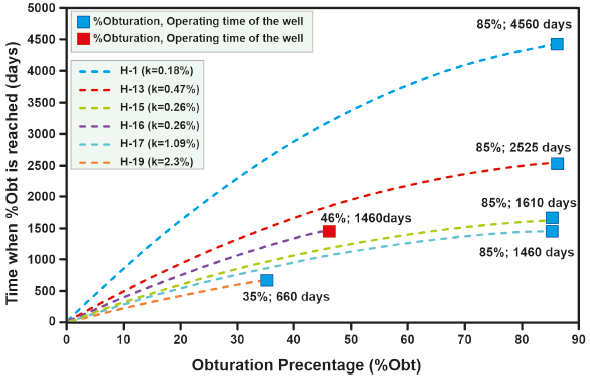
The time in which a certain percentage of seal is reached increases as the percentage of seal increases (Figure 14). In some wells, scale forms more quickly than in others; for example, wells H-15, H-16, H-17, and H-19 seem to reach a certain percentage of seal faster than wells H-01 and H-13. This has to do with the characteristics of each well. The results of this predictive model are validated by evaluating its performance by simulating wells H-24 and H-33, for which operating time data are available.
4.2. VALIDATION OF THE MODEL THAT PREDICTS THE FORMATION TIME OF AMORPHOUS SILICA SCALE
Cornejo (1996) provides information on the initiation and operational periods of wells H-24 and H-33. Both wells underwent direct modeling simulations, and the errors in predicting the time when scale formation occurs for H-24 and H-33 wells (as presented in Table 8) are below 3%. This demonstrates that the predictive model is accurate and effectively replicates the time at which well sealing occurs under the following conditions: 1) Temperatures within the range of 270°C to 305°C; 2) Enthalpies ranging from 1187 to 1400 kJ/kg; 3) Volumetric fractions of liquid
Table 7 Performance of the predictive model in the wells used for its validation.
| Well | Temperature (oC) |
Nto (mol) |
Diameter (m) |
W (kg/s) |
% Obt |
k | Time to reach % Obt Exp. (days) |
Time to Reach % Obt Model (days) |
Relative Error (%) |
|---|---|---|---|---|---|---|---|---|---|
| H-24 | 288.96 a | 1.3×10⁻⁴ | 0.21b | 5.5b | 85 | 0.72 c | 2735 b | 2663 | -2.63 |
| H-33 | 284.17 a | 5.9×10⁻⁵ | 0.17 b | 10b | 85 | 0.91 c | 1855 b | 1809 | -2.47 |
a) Calculated with the mathematical simulator; b) Cornejo 1996; c) Calculated by Equation 12.
Table 8 Projections of wells for which seal time information is not available.
| Well | Temperature (oC) |
Nto (mol) |
Diameter (m) |
W (kg/s) |
% Obt |
k | Time to Reach % Obt Model (days) |
|---|---|---|---|---|---|---|---|
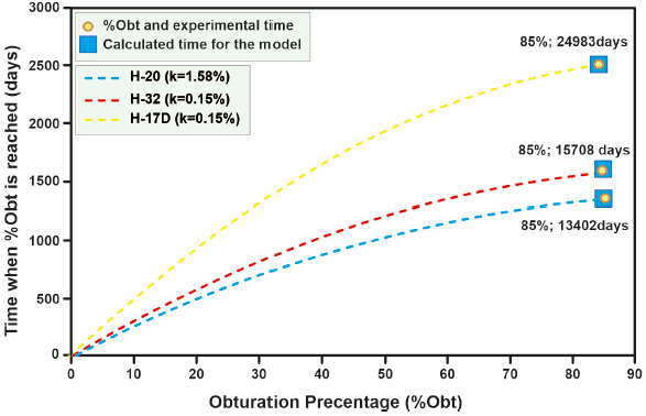
| H-17D | 278.61 a | 9.15×10⁻⁵ | 0.24 b | 5.5 c | 85 c | 0.15 d | 24983 |
| H-20 | 270.89 a | 4.20×10⁻⁶ | 0.17 b | 10.88 b | 85 | 1.58 d | 13402 |
| H-32 | 268 a | 8.05×10⁻⁵ | 0.24 b | 9.72 b | 85 | 0.15 d | 15708 |
a) Calculated with the mathematical simulator; b) Cornejo 1996; c) Aragón and Gonzales 2014; d Calculated by Equation 12.
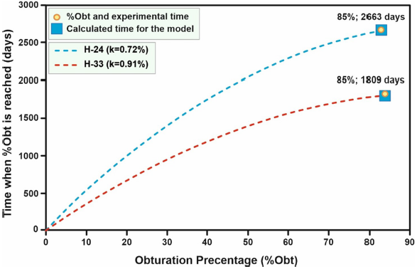
Figure 15 Changes in the percentages of sealing over time for the wells used in the validation of the correlation used to determine the parameter k.
5. Limitations
The proposed model for predicting amorphous silica obstruction in geothermal wells demonstrates promising potential within its defined scope. While its applicability may be more tailored to environments resembling Los Humeros, its specificity ensures a focused and accurate analysis in such contexts. The model's dependence on precise input parameters, although a limitation, underscores the importance of meticulous data collection for optimal performance. Seeing that the model only works with two-phase flow as a possible limitation makes it clear that we need to learn more about it and change it to work with situations where the fluids or flow patterns are different. Focusing on amorphous silica makes the model easier to use and helps with specific insights, even though it makes the mechanisms of scale formation simpler. Continuous efforts in ongoing research and validation endeavors are integral, serving as proactive measures to refine the model and extend its utility to a broader array of geothermal fields. The model's limitations, therefore, serve as stepping stones for improvement and evolution, contributing to the continuous advancement of predictive capabilities in geothermal well management.
6. Conclusion
The model developed in this study accurately predicts the point in time when pipe sealing reaches a certain percentage in wells. This prediction is reliable when volumetric fractions of liquid are high (εl > 5) and when temperatures remain within the range of 270 °C to 305 °C, with stable temperature, pressure, and enthalpy profiles over their production periods.
To enhance the performance of this model, we propose incorporating simulations that account for changes in pipe diameter due to amorphous silica accumulation. These changes influence temperature, pressure, and enthalpy at the depth where sealing occurs.
Our algorithm is highly sensitive to variations in mass flow and diameter, which have a significant impact on residence time calculations. Therefore, we recommend expanding the number of samples used in adjusting the 'k' parameter and introducing a term that considers the fluid's residence time in the pipe section.
In the case of well H-16, it was observed that the moles of amorphous silica precipitate more as the temperature increases, and differences were noted among solutions with pH values of 5.1, 7.7, and 8.9 at temperatures ranging between 280 °C and 300 °C. As the kinetic precipitation of amorphous silica is proportional to the residence time (the time it takes to fill the pipe), wider pipes and lower mass flows, such as those in Humeros, result in more significant amorphous silica deposition due to longer filling times.
Thermodynamic simulations were generated from adjustments of flow and heat models, producing accurate pressure and enthalpy profiles with errors between 1% and 15%. These simulations revealed that wells H-13, H-16, H-17, and H-19 draw from two reservoirs.
Wells fed from two reservoirs often encounter sealing and corrosion issues, leading to the maintenance-related closure of these wells. Upon reopening, these wells typically recover 75% of their production. Therefore, it is advisable to ensure that wells operate with a single reservoir feed whenever possible, as amorphous silica precipitates more readily in such wells, as observed in the behavior of wells H-13, H-16, H-17, and H-19.
The results obtained from simulating a diverse range of wells in the LHGF confirm the reliability and accuracy of the predictive precipitation model, with relative errors below 3%.
Early utilization of this type of model for characterizing production fields, in conjunction with traditional approaches, can positively influence the improvement of well construction characteristics and the implementation of preventive measures to mitigate mineral precipitation-induced clogging.
Declaration of competing interest
The authors declare that they have no known competing financial interests or personal relationships that could have appeared to influence the work reported in this paper.
Authors Contribution
All authors contributed to the study conception and design. Material preparation, data collection and analysis were performed by Sumit Mishra, Eduardo González-Partida, Sanjeet K. Verma, Kailasa Pandarinath, R. Pérez-Rodríguez, Joseph Madondo, and Antoni Camprubí. The first draft of the manuscript was written by Sumit Mishra, Eduardo González-Partida and all authors commented on previous versions of the manuscript. All authors read and approved the final manuscript.
Conflicts of Interest
The authors declare no potential conflict of interest.
Handling editor
Francisco J. Vega.
Data Availability Statement
The data that support the findings of this study are available from the corresponding author upon reasonable request.

