


 nueva página del texto (beta)
 Inglés (pdf)
 Artículo en XML
 Referencias del artículo
 Enviar artículo por email
 Citado por SciELO
  Similares en
SciELO
Similares en
SciELO 
 Permalink
1. INTRODUCTION
U Geminorum is the prototype of a subclass of dwarf novae (DN), which belong to the cataclysmic variable systems (CVs). These are semi-detached interactive binaries where the primary is a compact white dwarf (WD) accreting material from a Rochelobe filling companion, which normally is a late type star very close to the main-sequence. According to the classical model developed by Smak (1971) and Warner & Nather (1971), the material accreted by the secondary star forms an annulus or ring in the outer regions due to its large amount of angular momentum, and eventually forms a full disc, down to the boundary of the WD, due to viscous forces within its layers. When the disc is well formed the material strikes the disc in the outer rim which results in a conspicuous bright spot. This region, also known as the hot spot, is observed as an orbital hump in the optical light-curves of U Gem during quiescence, which precedes an eclipse of the bright spot and a partial eclipse of the accretion disc.
U Gem has an orbital period of 0.1769061911 days and a mass ratio of q = 0.35±0.05 (Echevarría et al. 2007), with an inclination of i = 69.7◦ ± 0.7◦ (Zhang & Robinson 1987). It has an outburst recurrence of ≈ 118 days. Models from Takeo et al. (2021) predict that the inner disc is truncated in quiescence at a distance of ≈ 1.20 − 1.25 times the WD radius, whereas in outburst it truncates at 1.012 R wd or might even extend to the WD surface. The FUV lightcurve analyzed by Godon et al. (2017) shows phase-dependent modulations which are consistent with a stream overflow of the disc.
Multiple radial velocity studies have been conducted on U Gem, from which the semi-amplitudes of the components have been derived. Tracing the Hα Balmer emission line, Echevarría et al. (2007) obtained a radial velocity for the white dwarf of K 1 = 107 ± 2 kms−1, in agreement with the analyses of FUV observations put forward by Long & Gilliland (1999), who reported a value of K 1 = 107.1 ± 2.1 kms−1.
By means of Doppler tomography - a technique that analyzes the Doppler shifts of an emission line to obtain a two-dimensional distribution of the emission in accretion discs (Marsh & Horne 1988)- this object has been observed to exhibit diverse emission structures in quiescence: from that of an extended disc dominated by the emission from the hot spot (Echevarría et al. 2007; Marsh et al. 1990), to a highly asymmetric shape similar to spiral arms overlaying the disc (e.g. Unda-Sanzana et al. 2006; Neustroev & Borisov 1998).
Despite being one of the best studied DN, and a prototype object, U Gem continues to show a behaviour far more complicated than that contemplated in the classical model. Thus, it is an object worth of continuous monitoring. With this in mind, in § 2 we present optical spectroscopic observations of U Gem obtained during quiescence. § 3 is a radial velocity study of the system implemented on three distinct emission lines: Hβ, Hγ, and Hδ, by means of which the masses of the system are derived. § 4 consists of the discussion of the derived masses. It also includes an extensive discussion on the Doppler tomography obtained for the emission lines, which we used to find clues on the spatial origin of the emission within the disc. Finally, our conclusions are presented in § 5.
2. OBSERVATIONS AND REDUCTION
Spectra were obtained with the 2.1-m telescope of the Observatorio Astrofísico Guillermo Haro at Cananea, Sonora, using the Boller and Chivens spectrograph and a E2V42-40, 2048x2048 CCD detector in the 4000 - 5000Å range with a resolution of R ≈ 1700, on the nights of 2021 February 15 and 16. The exposure time for each spectrum was 600s. Standard IRAF1 procedures were used to reduce the data.
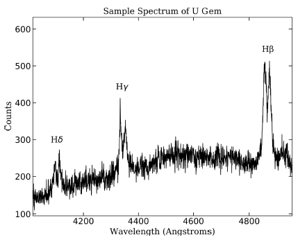
The log of observations is shown in Table 1. The spectra show strong double-peaked Balmer lines, as exhibited in the sample in Figure 1. The spectra are not flux calibrated, therefore the y-axis shows counts in each spectrum.
TABLE 1 LOG OF SPECTROSCOPIC OBSERVATIONS OF U Gem
| Date | Julian Date
(2450000 +) |
No. of
spectra |
Exp. Time |
| 15 Feb 2021 | 9260 | 47 | 600s |
| 16 Feb 2021 | 9261 | 34 | 600s |
3. RADIAL VELOCITIES
The radial velocity of the emission lines of each spectrum was computed using the RVSAO package in IRAF, with the CONVRV function, developed by J. Thorstensen (2008, private communication). This routine follows the algorithm described by Schneider & Young (1980), convolving the emission line with an antisymmetric function, and assigning the centre of the line profile to the root of this convolution. As in Segura-Montero et al. (2020), we used the DoubleGaussian method (GAU2 option available in the routine), which uses a negative and a positive Gaussian to convolve the emission line. The algorithm uses as input the width and separation of the Gaussians. This method traces the emission of the wings of the line profile, presumably arising from the inner parts of the accretion disc.
Following the methodology described by Shafter et al. (1986), we made a diagnostic diagram to find the optimal Gaussian separation, by fitting each trial to a simple circular orbit :
where γ is the systemic velocity, K 1 the semiamplitude (assumed to be the WD orbital velocity), t 0 the time of inferior conjunction of the donor and P orb is the orbital period. We employed χ 2 as our goodness-of-fit parameter. Note that we have fixed the orbital period in our calculations, and therefore we only fit the other three orbital parameters. This is a convenient way to improve the fit of the remaining free parameters as the orbital period has been obtained from the eclipses of the object (e.g. Echevarría et al. 2007).
Constructing a diagnostic diagram requires an interactive fitting between the CONVRV routine and a program to fit the orbital parameters. We have used ORBITAL2 a simple least squares program to determine, in general, the three free orbital parameters. In particular, a control parameter is defined in this diagnostic, σ K /K, whose minimum is a very good indicator of the optimal fit. In our runs we have found that the best results are obtained with a relatively small width of about 10-15 pixels. The diagnostic diagram for Hβ is displayed in Figure 2, while the orbital fit for its best solution is exhibited in Figure 3. The parameters yielded for the optimal orbital fit are shown in Table 2. In a similar way, we have constructed the diagnostic diagrams for Hγ and Hδ. These, and the corresponding best orbital fits, are shown in Figures 4 to 7, while the orbital parametrs are also shown in Table 2.
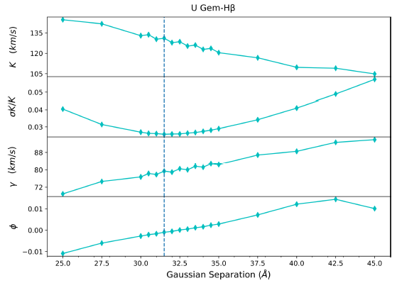
Fig. 2 Diagnostic diagram of the Hβ emission line. The vertical blue dashed line indicates the best solution. See text for further discussion. The colour figure can be viewed online.
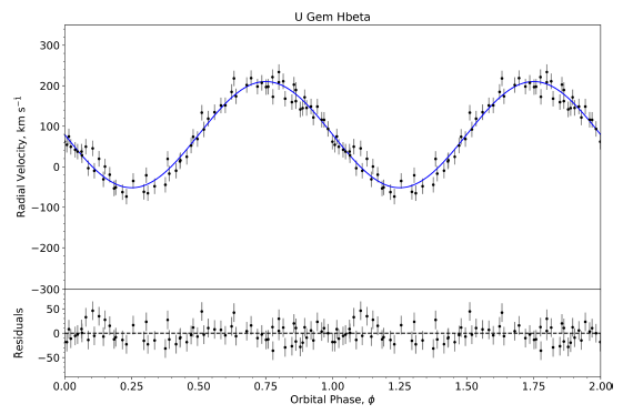
Fig. 3 Radial velocity curve for the best solution of the Hβ emission line. The colour figure can be viewed online.
TABLE 2 ORBITAL PARAMETERS
| Parameter | Hβ | Hγ | Hδ |
| γ (km s−1) | 79.4 ± 2.3 | 81.2 ± 3.4 | 122.5 ± 4.9 |
| K1 (km s−1) | 131.1 ± 3.3 | 110.0 ± 5.0 | 136.9 ± 7.1 |
| HJD0* | 0.0077 ± 0.0006 | 0.005 ± 0.001 | 0.008 ± 0.001 |
| Porb (min) | Fixed** | Fixed** | Fixed** |
*(2459261+ days).
**0.1769061911 days.
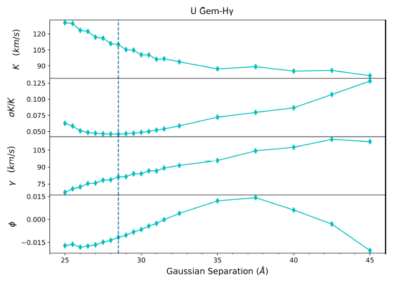
Fig. 4 Diagnostic diagram of the Hγ emission line. The vertical blue dashed line indicates the best solution. See text for further discussion. The colour figure can be viewed online.
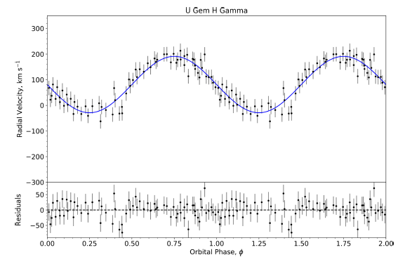
Fig. 5 Radial velocity curve for the best solution of the Hγ emission line. The colour figure can be viewed online.
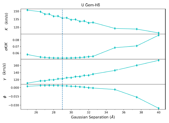
Fig. 6 Diagnostic diagram of the Hδ emission line. The vertical blue dashed line indicates the best solution. See text for further discussion. The colour figure can be viewed online.
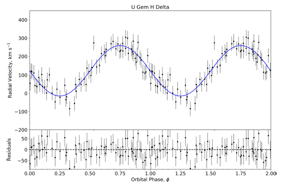
Fig. 7 Radial velocity curve for the best solution of the Hδ emission line. The colour figure can be viewed online.
The radial velocity fit for the Hβ and Hδ emission lines yield consistent K1 values within the errors. They also agree with the value of K1 = 138 ± 8 kms−1, obtained from an analysis of the same lines performed by Stover (1981). On the other hand Hγ agrees with the more accurate result of K1 = 107.1 ± 2.1 kms−1 obtained by Long & Gilliland (1999), who traced the Doppler shifts of the WD photospheric absorption lines in the FUV range; also in agreement with Echevarría et al. (2007), who followed the same methodology used in this paper, but applied to the Hα Balmer emission line only (K1 = 107 ± 2 kms−1).
4. DISCUSSION
4.1. Basic System Parameters
From the determination of the orbital parameters obtained in § 3 we can estimate the masses of the system components, as well as the binary separation, provided that an accurate estimation of the inclination angle is available. These mass estimates depend strongly on the assumption that the semiamplitude derived from the emission lines accurately reflects the motion of the white dwarf, i.e. that the measurements of the wings of the lines are not distorted and present a symmetric behavior along the orbital period. The basic system parameters are obtained with the following formulae:
where q is the mass ratio; M 1 is the mass of the primary; M 2 the mass of the secondary; i the inclination angle, K 1 and K 2 are the semi-amplitude of the primary and secondary, respectively; and a is the binary separation. To employ equations 2-5, we adopted the inclination derived by Zhang & Robinson (1987) of i = 69.7◦±0.7◦ and the semi-amplitude of the secondary derived by Echevarría et al. (2007) of K 2 = 310 ± 5 kms−1.
Table 3 shows a summary for the system parameters yielded when using each of the K 1 values from the three lines, obtained in § 3. For comparison, we also include the parameters reported for Hα by Echevarría et al. (2007).
TABLE 3 BASIC SYSTEM PARAMETERS YIELDED BY THE K1 AMPLITUDE VALUE OF EACH EMISSION LINE
| Parameter | Hα† | Hβ | Hγ | Hδ |
| q | 0.34 ± 0.01 | 0.42 ±0.01 | 0.35 ±0.01 | 0.44 ±0.02 |
| M1 (M ⊙) | 1.20 ± 0.05 | 1.34 ±0.05 | 1.22 ±0.06 | 1.38 ±0.07 |
| M2 (M ⊙) | 0.42 ± 0.04 | 0.57 ±0.02 | 0.43 ±0.03 | 0.61 ±0.05 |
| α(R⊙) | 1.55 ± 0.02 | 1.64 ±0.02 | 1.56 ±0.03 | 1.67 ±0.03 |
As expected from the high K 1 values for Hβ and Hδ, and because we are using the same i and K 2 constraints as Echevarría et al. (2007), the system parameters for these lines resulted in an overestimation with respect to those obtained from the Hα analysis of the aforementioned authors (See Table 3). On the other hand, the parameters yielded for Hγ are consistent with those reported by Echevarría et al. (2007), because of the agreement of the K 1 value.
A possible explanation for our radial velocity parameter overestimation and thus for our mass parameter calculations could be made based on the X-ray analysis of Takeo et al. (2021), whose models predict that the accretion disc is truncated at 1.25 Rwd during quiescence, as expected by the theory (Narayan & Popham 1993). Given that the Double-Gaussian method, employed in § 3, traces the inner region of the disc, this truncation could result in higher values for the radial velocity of the WD.
It is possible that the inner part of the disc does contain mass, but at such low density and low surface brightness that it is optically thin (e.g. Pringle 1981). Furthermore, as explained in § 4.2, we detect an asymmetry overlaying the disc in our Doppler tomograms. These circumstances could imply abrupt variations of opacities within the disc, which would explain our internal inconsistencies in the radial velocity analysis (e.g. Mason et al. 2000).
4.2. Doppler Tomography
Doppler tomography is an indirect imaging technique developed by Marsh & Horne (1988). It produces two-dimensional mappings of the emission intensity in velocity space of the accretion disc, using the phase-resolved profiles of the spectral emission lines. We produced the Doppler tomography of the Hβ, Hγ and Hδ Balmer emission lines, using a Python wrapper 3 (Hernandez Santisteban 2021) of the fortran routines published by Spruit (1998) within an IDL environment. Figures 8-10, show the resulting images from the analysis, with the following layout: in the top left panel we show the observed trailed spectra; the tomography is displayed in the bottom panel; and the reconstructed trailed spectra, which are created by collapsing the tomography image along the direction defined by the respective orbital phase (Marsh 2005), appear in the top right panel.
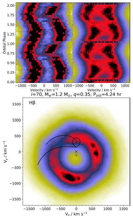
Fig. 8 Trail spectra and Doppler tomography of the Hβ emission line. The relative emission intensity is shown in a scale of colours, where the strongest intensity is represented by black, followed by red, then blue, and finally yellow. The cross markings represent (from top to bottom) the position of the secondary, the centre of mass and the primary component. The Roche lobe of the secondary is depicted around its cross. The Keplerian and ballistic trajectories of the gas stream are marked as the upper and lower : curves, respectively. The colour figure can be viewed online.
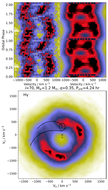
Fig. 9 Trail spectra and Doppler tomography of the Hγ emission line. The relative emission intensity is shown in a scale of colours, where the strongest intensity is represented by black, followed by red, then blue, and finally yellow. The cross markings represent (from top to bottom) the position of the secondary, the centre of mass and the primary component. The Roche lobe of the secondary is depicted around its cross. The Keplerian and ballistic trajectories of the gas stream are marked as the upper and lower curves, respectively. The colour figure can be viewed online.
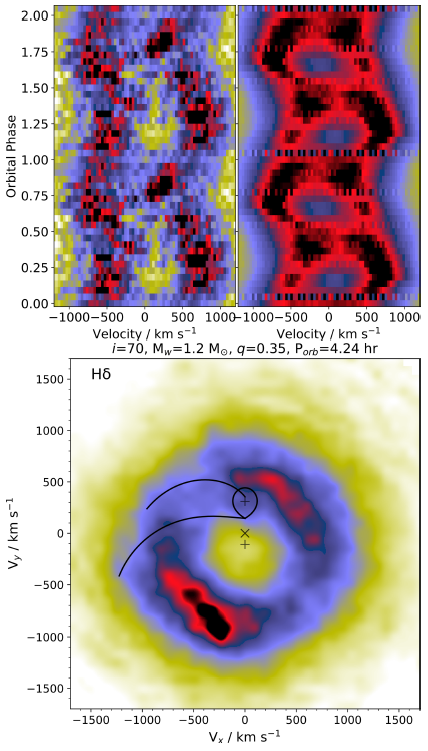
Fig. 10 Trail spectra and Doppler tomography of the Hδ emission line. The relative emission intensity is shown in a scale of colours, where the strongest intensity is represented by black, followed by red, then blue, and finally yellow. The cross markings represent (from top to bottom) the position of the secondary, the centre of mass and the primary component. The Roche lobe of the secondary is depicted around its cross. The Keplerian and ballistic trajectories of the gas stream are marked as the upper and lower curves, respectively. The colour figure can be viewed online.
The trailed spectra of all three Balmer lines show a conspicuous double-peaked structure, characteristic of the line profiles of discs in systems of high inclination (Horne & Marsh 1986; Marsh & Horne 1988). The spectrograms exhibit an evident lack of a hot-spot signature, which would appear as an s-wave oscillating from peak to peak.
The overall structure in our three tomography images is in contrast to most previous Doppler tomography studies of U Gem in quiescence, which were dominated by an intense emission corresponding to a hot spot component (e.g. Marsh et al. 1990; Echevarría et al. 2007). Instead, we find an asymmetric region of enhanced emission overlaying the disc, consistent with the structure exhibited by spiral density waves (eg. Steeghs et al. 1997). While U Gem has been observed to show this structure in Doppler tomograms before (Neustroev & Borisov 1998; Unda-Sanzana et al. 2006), the presence of fully formed spiral shocks in U Gem must be regarded with caution: the study of the evolution of spiral shocks in U Gem performed by Groot (2001) shows that they fade during the decline of the outburst. And even if spiral arms were present in U Gem in quiescence, they would be expected to be tightly wrapped during this stage (Steeghs & Stehle 1999); hence very difficult to detect with Doppler tomography (Ruiz-Carmona et al. 2020). As discussed by Unda-Sanzana et al. (2006), the spiral feature in the tomography could instead be explained by irradiation from the WD of regions of the disc that become thickened from tidal distortion.
Nonetheless, our understanding of spiral shocks from 2D models has shown limitations before, as in the simulations by Godon et al. (1998) which predicted an unrealistically hot disc in order to reproduce the two-armed spiral pattern exhibited in the tomography of IP Peg by Steeghs et al. (1997). Moreover, a previous detection in quiescence makes the limitations evident: the Doppler maps reported by Pala et al. (2019) exhibit a clear signature of spiral shocks in a quiescent state of the WZSge object SDSSJ123813.73-033933.0; confirmed by the double hump modulation of the white dwarf in their HST data, caused by the interface between the white dwarf and the inner edge of the spiral shocks. And since the mass ratio of U Gem, q = 0.35 ± 0.03 (Echevarría et al. 2007), sets it right on the limit that allows the disc to achieve the 3:1 resonance (q ≲ 0.3) (Hellier 2001), spiral arms cannot be completely discarded.
Another possible explanation is provided by Smak (2001), who argues that the high radial velocity of K 1 = 138±8 kms−1 obtained by Stover (1981) (in accordance with our own values yielded for Hβ and Hδ) could be caused by stream overflow of the disc. This would explain the absence of a hot spot in our tomography images, since the stream overshoot would avoid (or ameliorate) the initial impact with the rim of the disc. Stream material overshooting the disc edge and re-impacting at radii with lower velocity can create a second hot spot (Lubow 1989) which usually shows up in regions within the lower quadrants of the Doppler tomograms, as is the case in SW Sextantis systems (Schmidtobreick 2017). This scenario is further supported by the phase-dependent modulation of the FUV light curve and absorption lines velocity reported by Froning et al. (2001), which can be explained by the stream overflowing the edge of the disc (Godon et al. 2017; Godon 2019).
In any case, it is puzzling that our tomography shows similar emission distributions for all three emission lines, implying that they arise from the same regions in the disc. This raises the question: why is it that for Hβ and Hδ we obtain values that are consistent with Stover (1981), which are likely corrupted by some additional effect on the disc; while on the other hand Hγ appears unaffected and agrees better with the more reliable WD radial velocity measured from HST FUV observations by Long & Gilliland (1999)? As mentioned in § 4.1, we expect this internal inconsistency to be caused by different gas opacities in the accretion disc (Mason et al. 2000), occurring as a consequence of some combination of the phenomena discussed above: WD irradiation of tidally thickened regions, stream overflow, a partially truncated disc, and perhaps even fully formed spiral arms.
However, this inconsistency is a clear example of the issues arising from measuring the radial velocity of the WD from optical data, even when presumably tracing the inner regions of the disc as is done in the Double-Gaussian method (see § 3).
5. CONCLUSIONS
We presented a spectroscopic analysis of the dwarf nova U Geminorum. We obtained the radial velocity of the system for three distinct Balmer emission lines: Hβ, Hγ, and Hδ, by tracing the outer regions of the profile (which arise from the inner sections of the accretion disc), with the purpose of obtaining the WD radial velocity K 1. The resulting semi-amplitude for Hγ is consistent with previous canonic results of K 1 = 107.1±2.1 kms−1 (Echevarría et al. 2007; Long & Gilliland 1999). However, the other two lines show a considerable discrepancy, agreeing instead with the value obtained by Stover (1981) of K 1 = 138 ± 8 kms−1. We expected to find the source of this inconsistency in the Doppler tomography study, but the tomograms show that all three lines arise from the same region. However, it must be noted that the tomography does not show a typical disc: in particular there is no evidence whatsoever of a hot spot; instead it exhibits a spiral arm structure unexpected for a system in quiescence. This unusual shape (which can be a product of stream overflow, WD irradiation or actual spiral arms), along with a partial truncation of the inner regions of the disc, could together amount to considerable differences of gas opacities within the accretion disc, which could explain the different values of K 1 obtained for our three emission lines (e.g. Mason et al. 2000).
U Gem stands as one of the best studied DN. However, as it is made evident in this paper, more ingredients than those prescribed by the classical model must come into play to better explain its behaviour. Therefore, we propose further observations of this source to help shed light on the mechanisms giving rise to its rich and interesting nature.

