Appendix

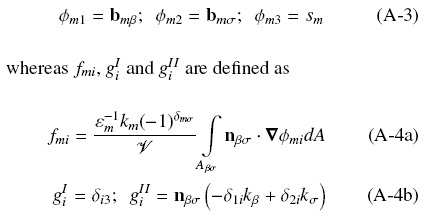
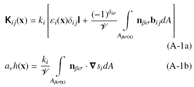
In this section, the definitions of the eective transport properties involved in Eqs. (3) and (5) and the closure problems for predict them are presented. The closure scheme involves a long theoretical procedure and was recently reported by Aguilar-Madera et al. (2011) (see details in their Appendix). The efective transport properties are given by the following compact formulation,

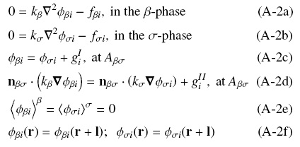
Here the subscripts i and j can be β or σ, δ_ij is the Kronecker's delta, | is the identity tensor, A_βσ is the interface fluid-solid location and n_βσ is the unit normal vector pointing from the fluid to the solid. b and s are the so-called closure variables solving the following steady-state boundary-value problems: Problem i, i = 1; 2; 3

where φ_mi (m = β,σ) represents scalar and vectorial variables according to