
Appendix 2
This appendix presents the evidence of the volatility and correlation clustering in the six markets (benchmarks) of the investment policy in Table 1. In order to test the presence of the volatility clustering, the Engle’s ARCH test (Engle, 1982) was performed in each asset and in each of the weekly dates used in the discrete event simulations. A 95% confidence level is used to test the next hypothesis:
H0 : T · R2 > X295%,T (2.1)
Where R2 is the coefficient of determination of the next auxiliary regression given
ε2t = α + βiε2t-i (2.2)
This test was performed in each weekly date used for the simulation from January 2, 2002 to December 31, 2010.19 The results are presented in Chart A2.1 and the number of dates with a presence of the ARCH effect is resumed in Table A2.1.
As noted in Chart A2.1, not all the dates presented an ARCH effect, sug-gesting that not in all of them an OGARCH matrix should be used in the MTSL
model. In order to accept a general use of GARCH models in all the dates, a Poisson probability function hyphotesis test is used by using a mean of λ = 23 and
a 95% confidence level given by λ + (95% · λ) = 28.10. With these parameters, the number of dates that report the presence of the ARCH effect are compared, and if this number was higher than 28.10, the presence of the ARCH effect was accepted for all the dates by assuming that the number of dates is high enough to generalize the presence of this phenomenon in each asset.
The results of these hypothesis tests are presented in the right panels of Chart A2.1 and Table A2.1. It can be shown that almost all the benchmarks (excepting the us treasuries -EFFAUSB100- that is not conclusive) lead to the acceptance of the ARCH effect for all dates.


Once the evidence of the ARCH effect in the six benchmarks is presented, it is necessary to prove the usefulness of an OGARCH covariance matrix by testing the presence of the correlation clustering effect. In order to do so, the return time series rt in each asset was divided in two time groups by using the next distance suggested by Chow, Kritzman and Lowry (1999):

Where rt is a 6 x 1 vector with the observed return at date t in each asset,  is a vector with the means of the entire time series rt in each asset and C0 the covariance matrix for the same data:

Each date t or returns vector rt was included in the "unusual dates" set Θ by following the next rule:

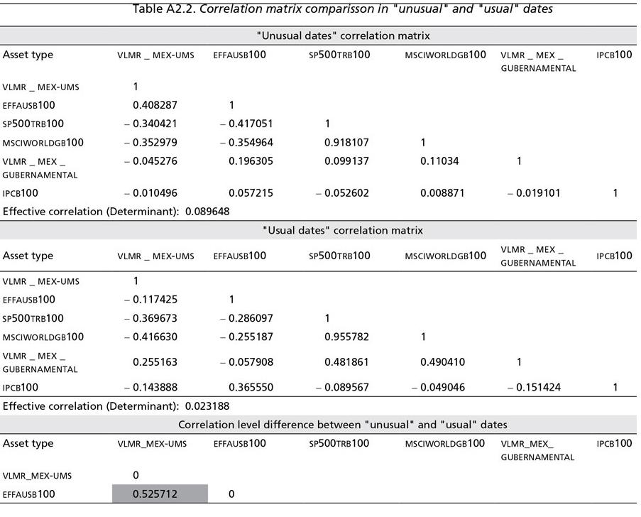
Where v are the degrees of freedom related to the number of assets included in the covariance matrix C0. Once Θ and ΘC are defined by equation (2.5), two correlation matrixes were calculated for the usual and unusual date sets and the correlation of ΘC was rested to the one of Θ, leading to the results of Table A2.2.
As can be noted, the correlation observed in "unusual times" increased in eight of 15 pairs of assets (or markets), suggesting the presence of correlation clustering in turbulent or unusual times. This can also be observed in the difference of the effective correlation (determinant) value between both matrixes.
19 Por supuesto, la devolución de impuestos a las familias, las ofertas por parte de las tiendas comerciales, como el Black Friday, la reducción de impuestos a los productores y la recapitalización de las instituciones financieras fueron acciones que actuaron en la misma dirección. Es decir que el programa de medidas correctivas del gobierno estadounidense mezcló políticas fiscales con políticas monetarias; no se trató, por tanto, de un programa de rescate exclusivamente keynesiano, como ha tendido a argumentarse.