APPENDIX 2

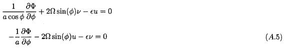
While all the cases in the main part of the paper use a rectangular region it may be of interest to consider a single case using spherical geometry. The two equations of motion are then in the steady state as given in (A.5).

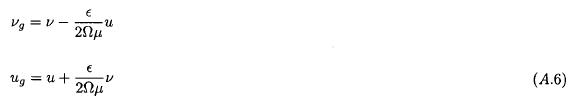
By using the definition of the geostrophic wind components one may rewrite (A.5) in the form given in (A.6) with m = sin(j).

Comparing first the wind speeds we obtain from (A.6) the relation given in (A.7).

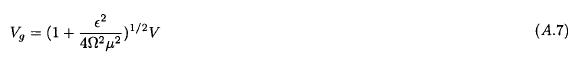
Since the second term in the parenthesis is about 7.5 x 10^–4 at any of the poles we find that V_g = 1.0007 V indicating that geostrophy exists with excellent approximation close to the poles. On the other hand, at low latitudes, say μ = 0.1, we find that V_g = 1.0370V, while μ = 0.01 leads to V_g = 2.92 V. (A.7) and the examples show the well known fact that geostrophy is a good approximation in the middle and higher latitudes.

One may also compare the directions of the wind and the geostrophic wind. From (A.6) we obtain (A.8).

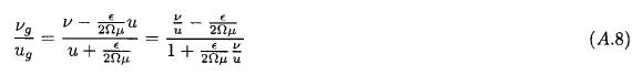
If v = 0 (zonal wind) we find that v_g / u_g = —0.03/m showing that the geostrophic wind has a small southward component in middle and higher latitudes, or that the effect of friction is to create a cross-isobaric flow. In the case v/u = 1 it is seen from (A.8) the geostrophic ratio v_g / u_g becomes smaller than unity.