Articles
Evaluating the Impact of Removing Low-relevance Features in Non-retrained Neural Networks

-
Publication dates-
January 21, 2025
Jul-Sep , 2024
- Article in PDF
- Article in XML
- Automatic translation
- Send this article by e-mail
- Share this article +
Abstract:
Feature selection is a widely used technique to boost the efficiency of machine learning models, particularly when working with high-dimensional datasets. However, after reducing the feature space, we must retrain the model to measure the impact of the removed features. This can be inconvenient, especially when dealing with large datasets of thousands or millions of instances, as it leads to computationally expensive processes. To avoid the costly procedure of retraining, this study evaluates the impact of predicting using neural networks that have not been retrained after feature selection. We used two architectures that allow feature removal without affecting the architectural structure: FT-Transformers, which are capable of generating predictions even when certain features are excluded from the input, and Multi-layer Perceptrons, by pruning unused weights. These methods are compared against XGBoost, which requires retraining, on various tabular datasets. Our experiments demonstrate that the proposed approaches achieve competitive performance compared to retrained models, especially when the removal percentage is up to 20%. Notably, the proposed methods exhibit significantly faster evaluation times, particularly on large datasets. These methods offer a promising solution for efficiently applying feature removals, providing a favorable trade-off between performance and computational costs.
Keywords::
Feature selection, transformers, pruning models, neural networks
1 Introduction
Collecting data is an extensive process that corporations employ to extract knowledge and enhance process efficiency [15]. This has resulted in the creation of large databases, presenting an opportunity to apply machine learning and deep learning techniques, which thrive on substantial amounts of data for achieving remarkable results. Nevertheless, the collected data may contain several variables, causing the creation of high-dimensional datasets.
-
15Customer data: Designing for transparency and trustHarvard Business Review, 2015
When dealing with high-dimensional information, many challenges and complications arise, such as an exponential increase in computational effort, large waste of space, poor visualization capabilities, and the inability of machine learning algorithms to manage this data [20, 18].
-
20The curse of dimensionality: Inside out, 2018
-
18Artificial Intelligence: A Modern Approach, 2010
Even though including more variables may theoretically allow for the storage of more information, this may not be beneficial in practice. This is due to the higher likelihood of encountering noisy and redundant information in the dataset [20, 14]. A straightforward approach for dealing with high-dimensional data is to remove features that have repeated information or constant values.
-
20The curse of dimensionality: Inside out, 2018
-
14Applied Predictive Modeling, 2013
This type of data cleansing is a natural part of the process. However, we may also need to reduce features that are still important to the problem, but not as essential as others. To achieve this, it is common to employ a feature selection algorithm. These algorithms help us reduce the number of features to a desired size, but they use complex rules to determine which features to remove. This allows us to streamline the dataset while retaining the most relevant information. Evaluating the quality of a feature subset can be computationally expensive. The process typically involves the following steps:
-
Train an initial model using all available features to establish a baseline performance metric (e.g., accuracy).
-
Apply a feature selection algorithm to create a subset of the features. Once the relevant features are selected.
-
Train a second model using this reduced feature set, and finally.
-
Compare the performance of the two models. If the performance degradation between the two models is unacceptable, you must repeat the process.
This may involve trying a different feature selection algorithm or tuning the parameters of the current feature selection algorithm (e.g., changing the size of the generated subset). This iterative process of training models with different feature subsets to evaluate their quality can be computationally expensive.
The most prominent models for tabular data are tree-based algorithms, such as XGBoost, and neural networks [4, 9, 10, 13, 11, 7]. When dealing with large datasets, these models can take a significant amount of time to train. This poses a challenge when evaluating feature subsets generated by selection algorithms. Performing multiple iterations of training models with different feature subsets can be disadvantageous due to the computational expense.
-
4XGBoost: A scalable tree boosting system, 2016
-
9Random decision forests, 1995
-
10TabPFN: A transformer that solves small tabular classification problems in a second, 2022
-
13Well-tuned simple nets excel on tabular datasets, 2021
-
11TabTransformer: Tabular data modeling using contextual embeddings, 2020
-
7Revisiting deep learning models for tabular data, 2021
To address the challenge of the computationally expensive process of evaluating feature subsets, this study explores the use of two neural network architectures as final predictive models. The key advantage is that these models do not require retraining when low-relevance features, as identified by feature selection algorithms, are removed. The first architecture is a multi-layer perceptron (MLP), where the weights of the removed features are pruned.
The second architecture is the FT-Transformer [7], which allows the model to generate predictions even when the embeddings of certain features are excluded from the input. Our findings show that these neural network models can perform competitively even without the need for retraining. When we removed up to 60% of low-relevance features, we observed performance degradations of less than 10%.
-
7Revisiting deep learning models for tabular data, 2021
Crucially, by avoiding retraining, we were able to speed up the decision-making process by up to 300 times compared to the iterative training approach, especially for large datasets. Furthermore, we discovered that using up to 20% of the low-relevance features, the non-retrained neural networks could be employed as final predictive models without significant performance loss compared to retraining-based methods. The main contributions of this study are as follows:
-
We introduce a straightforward pruning rule for MLPs when removing features.
-
We conduct a comparison of the proposed neural network architectures against retraining XGBoost, one of the most prominent models for tabular data. This comparison allowed us to determine the degradation rate and the evaluation speed when reducing the number of features across seven datasets.
-
We show that non-retrained neural networks remain competitive, achieving a degradation rate of less than 10% even when features are removed.
-
We demonstrate that pruned MLPs can be up to 300 times faster than tree-based methods when evaluating the impact of feature reduction.
-
We show that decision trees as feature selection algorithms generally achieve a small degradation rate.
The remainder of this paper is organized as follows: Section 2 provides background on the feature selection techniques and their considerations. In Section 3, we introduce the pruning rule for the MLPs. Additionally, we explain why the FT-Transformer has the ability to produce predictions even when features are removed.
Section 4 details the models selected for comparison and their optimization process. It also describes the datasets employed and their preprocessing. Finally, we outline the feature selection procedure used. Section 5 presents the performance degradations and execution times achieved by each approach, demonstrating the benefits of the proposed methods. Finally, Section 6 summarizes the key findings.
2 Background
Feature selection refers to the process of determining which features should be included in a model. From a practical standpoint, a model with fewer features can be more interpretable and less expensive to operate [14]. For example, a neural network with a lower number of features requires fewer parameters. Similarly, a tree-based model with fewer features requires fewer splits, resulting in shallower trees.
-
14Applied Predictive Modeling, 2013
These model reductions lead to faster training and inference times, directly impacting the computational costs, whether in terms of time or monetary expense (e.g., when performed in a cloud environment).
Another perspective is that if a variable requires high-precision equipment to measure, and it is not as relevant as other features, we can discard its measurement, thereby saving costs. This highlights how feature selection can optimize the model complexity and the data collection process. The feature selection methods are classified into three types [17]:
-
17A review of feature selection methods for machine learning-based disease risk predictionFrontiers in Bioinformatics, 2022
-
Filter Methods. Rank the features based on their scores in various statistical tests for their correlation with the prediction target. The top-ranked features are kept, while the others are removed.
-
Some key benefits of filter methods are that they are independent of the model used, are fast and scalable, capture feature dependencies, and reduce the overfitting risk.
-
A simple approach is to rank the features based on their linear correlation with the target variable. The features with the highest correlation are placed at the top of the ranking.
-
-
Wrapper Methods. Identify the best performing set of features for a specific model by using the model’s own performance as the metric to guide the selection of the optimal feature subset [8]. This is why wrapper methods typically outperform filtering methods regarding model performance, being its main advantage [12, 2, 6]. One example of a wrapper feature selection method is the F-Test.
-
This approach creates a candidate linear model by removing a feature, and then statistically compares the similarity between the error means when using all features versus when one feature is removed, using an F-score. If the difference in error means is not statistically significant, the removed feature is considered non-relevant [22, 14].
-
-
Embedded Methods. Integrate the feature selection process directly into the model. During the training step, the model determines the relevance of each feature through its parameters or decision steps, to achieve the best evaluation score.
-
Once the model is trained, the importance of each feature can be recovered and ranked to perform the feature selection. Embedded methods are faster than wrapper methods, as they only require a single training phase.
-
One example of an embedded method is using a decision tree, where the feature importance is computed as the normalized total reduction in the Gini index brought about by that feature [23]. Another approach is to use the coefficients of a linear model, where a feature’s importance is determined by its coefficient’s magnitude, as long as the features are properly normalized [22].
-
-
8An introduction of variable and feature selectionThe Journal of Machine Learning Research, 2003
-
12Filter versus wrapper gene selection approaches in DNA microarray domainsArtificial Intelligence in Medicine, 2004
-
2Feature selection methods: Case of filter and wrapper approaches for maximising classification accuracyPertanika Journal of Science and Technology, 2018
-
6A wrapper-filter feature selection technique based on ant colony optimizationNeural Computing and Applications, 2019
-
22Introductory econometrics: A modern approach, 2013
-
14Applied Predictive Modeling, 2013
-
23Ensemble machine learning: Methods and applications, 2012
-
22Introductory econometrics: A modern approach, 2013
Each feature selection method has its own benefits and drawbacks when compared to the others. As a result, no single algorithm can be considered universally optimal for all problems. This is why exploring and utilizing various feature selection methods is generally encouraged. However, it’s important to carefully consider the trade-offs between the effectiveness and efficiency of each approach.
3 Methodology
In this section, we outline the approaches taken to avoid retraining neural networks when relevant features are removed. We explain the pruning rule applied to a Multi-layer Perceptron (MLP). This approach allows us to efficiently update the model when removing less relevant features, without the need for full retraining.
Next, we briefly describe the FT-Transformer architecture and its ability to generate predictions even when the embeddings of certain features are excluded from the input.
This property of the FT-Transformer enables feature removals without any changes to the model structure or the need for retraining. The key benefit of these approaches is the ability to quickly assess the impact of removing low-relevance features, without the overhead of retraining the entire model for each feature subset evaluation.
3.1 Pruned Multi-Layer Perceptron
The Multi-layer Perceptron (MLP) is a fundamental approach for tabular data. It consists of a composition of affine transformations, including non-linearities, to create complex decision boundaries or simulate complex behaviors. The first layer of an MLP using a ReLU non-linearity can be expressed as:
e1ReLU ( W x + b ) ∈ ℝ h ,
where
It is, for a subset of features
This keeps the output dimension
e2ReLU ( W ⋅ , ℱ X ℱ + b ) ∈ ℝ h .
This pruning approach allows us to efficiently update the MLP model when removing less relevant features, without the need for full retraining.
3.2 FT-Transformer
The FT-Transformer [7] is an approach that combines a Feature Tokenizer with a Transformer architecture for tabular data. It creates embeddings for numerical and categorical variables (feature tokenization process) processed by a Transformer [19] variant. For numerical features, the embedding process involves applying an independent Multi-Layer Perceptron (MLP) to each feature.
-
7Revisiting deep learning models for tabular data, 2021
-
19Attention is all you need, 2017
For categorical features, the embedding process consists of applying an ordinal encoding to each feature and creating a look-up table for each one, similar to the approach used in Natural Language Processing tasks [19, 5]. Once tokenized, the embeddings are combined with an additional classification token [CLS] [5] at the beginning of the sequence.
-
19Attention is all you need, 2017
-
5BERT: Pre-training of deep bidirectional transformers for language understanding, 2018
-
5BERT: Pre-training of deep bidirectional transformers for language understanding, 2018
This sequence is then processed by a Transformer encoder variant, which includes a PreNorm layer [21] and removes the first normalization from the first Transformer layer. Finally, the output embedding corresponding to the [CLS] token is passed through layer normalization [1], a ReLU activation function, and a single-layer perceptron with an identity activation function to make predictions.
-
21Learning deep transformer models for machine translation, 2019
-
1Layer normalization, 2016
The FT-Transformer’s capacity to generate predictions even when the embeddings of certain features are excluded from the input is enabled by its Multi-head Self-Attention (MHSA) mechanism as follows:
Let’s consider the input to the FT-Transformer as a matrix of embedded features
The MHSA computation for a single layer of the FT-Transformer can be expressed as:
e3Softmax ( ( E W Q ) ( E W K ) T d ) ( E W V ) ∈ ℝ ( m + 1 ) × d ,
where usually,
However, the output of the MHSA and the output of the Transformer encoder will now have a dimension of
4 Experiments
This section outlines the experimental setup used to evaluate the impact of removing low-relevant features on non-retrained neural networks. We begin by describing the approaches taken for the model evaluation and optimization processes.
Next, we provide details on the datasets used in the study, as well as the data preprocessing steps applied. Finally, we outline the feature selection procedure that was followed, including the specific algorithms employed.
4.1 Compared Approaches
To compare the performance degradation of the Pruned MLP and FT-Transformer models when removing low-relevance features without retraining, we employed the XGBoost [4] algorithm as a baseline. The comparisons were made by removing features in increments of 10%, from 100% of the features down to 40%.
-
4XGBoost: A scalable tree boosting system, 2016
For the neural network models, we first performed a hyperparameter search using the full set of features, employing a grid search strategy. We then kept the architecture with the highest balanced accuracy fixed, and applied the pruning rules described in Section 3 for each feature removal scenario.
For the XGBoost models we took two approaches. The first (XGBoost) perform an initial grid search using the full feature set, then keep the highest performing architecture fixed for each feature removal, retraining the model.
The second approach (XGBoost + HS) performs the hyperparameter search for each subset of features tested. All models were optimized using the cross-entropy loss. The neural networks used the AdamW optimizer for 150 epochs with 30 early stopping patience steps. The XGBoost models were trained over 150 estimators with 30 early stopping patience steps. The hyperparameter search spaces for each model are described in Table 1.
Table 1
Hyperparameter search space for models selected for comparison
Hyperparameter search space for models selected for comparison
| Model | Hyperparameter | Search set |
| FT-Transformer | Embedding dimension | {128, 256} |
| Number of heads | {4, 8, 16, 32} | |
| Number of layers | {2, 3, 4, 5} | |
| Attention dropout | {0.3} | |
| Point-wise neural network dropout | {0.1} | |
| Learning rate | {10-4} | |
| Weight decay | {10-4} | |
| MLP | Hidden layers | {3, 6} |
| Hidden units | {512} | |
| Attention dropout | {0.3} | |
| Dropout | {0.2} | |
| Learning rate | {10-3} | |
| Weight decay | {0.1} | |
| XGBoost | Maximum depth | {5, 10, 15, 20} |
| Learning rate | {0.1} |
4.2 Datasets and Preprocessing
We selected seven datasets from the OpenML repository [3]. The selected datasets were: volkert, jasmine, nomao, kr-vs-kp, sylvine, australian, and adult. The properties of these datasets are summarized in Table 2.
-
3OpenML: An R package to connect to the machine learning platform OpenMLComputational Statistics, 2017
Table 2
Properties of selected datasets. Datasets are sorted by their number of features
Properties of selected datasets. Datasets are sorted by their number of features
| Dataset | # Features | # Instances |
| volkert | 181 | 58310 |
| jasmine | 145 | 2984 |
| nomao | 119 | 34465 |
| kr-vs-kp | 37 | 3196 |
| sylvine | 21 | 5124 |
| australian | 15 | 690 |
| adult | 15 | 48842 |
The datasets were split into 80% for training and 20% for testing. The training partition was further divided into five stratified folds to perform cross-validation (CV). Numerical features were normalized to have a mean of 0 and a standard deviation of 1. Missing values were imputed using the KNNImputer from scikit-learn [16] with
-
16Scikit-learn: Machine learning in PythonJournal of Machine Learning Research, 2011
For the FT-Transformer and XGBoost models, categorical features were encoded using an ordinal encoder, where the zero code was reserved for null values. In contrast, the MLP model used one-hot encoding for the categorical features.
4.3 Feature Selection
We considered three approaches for feature selection: the F-test, the decision tree, and linear model embedded methods. While embedded methods are particularly well-suited when applying feature reduction directly to the model that embeds the feature relevance, their feature ranking can still be leveraged and applied to other models as well. We used a specific methodology to perform the feature selection. First, we standardized the numerical features to have a mean of 0 and a standard deviation of 1, and one-hot encoded the categorical features. All missing values were replaced with zeros. Next, we performed feature selection using each of the three algorithms.
When a feature was selected among the top
This selection process continued until
5 Results
5.1 General Performance
We verify that every proposed method achieves similar results for every dataset when training using the entire set of features. This is because if the proposed methods were not competitive in the first instance, they would be discarded as an initial model. Table 3 shows the balanced accuracy in the test set for the fixed architectures from the cross-validation scores. Due to the selection methodology, the XGboost and XGBoost + HS models are the same when training using all characteristics.
Table 3
Test balanced accuracy for each considered method when training in the whole set of features
Test balanced accuracy for each considered method when training in the whole set of features
| Dataset | FT-Transformer | MLP | XGBoost |
| volkert | 63.578 | 60.139 | 59.494 |
| jasmine | 80.477 | 77.255 | 80.560 |
| nomao | 94.813 | 94.010 | 96.217 |
| kr-vs-kp | 99.685 | 99.211 | 97.348 |
| sylvine | 94.123 | 92.955 | 94.689 |
| australian | 85.448 | 86.129 | 89.067 |
| adult | 79.187 | 78.774 | 76.816 |
5.2 Performance and Efficency
The removal of low-relevant features can affect the models in two ways. First, the information reduction may impact the models’ performance. Second, the models may become more efficient, as they require fewer parameters and operations.
To evaluate these trade-offs, we assess the benefits and disadvantages of using non-retrained networks in both aspects. Figure 1 presents two cases of study: the volkert and adult datasets, which have the highest and lowest number of features, respectively.
Thumbnail
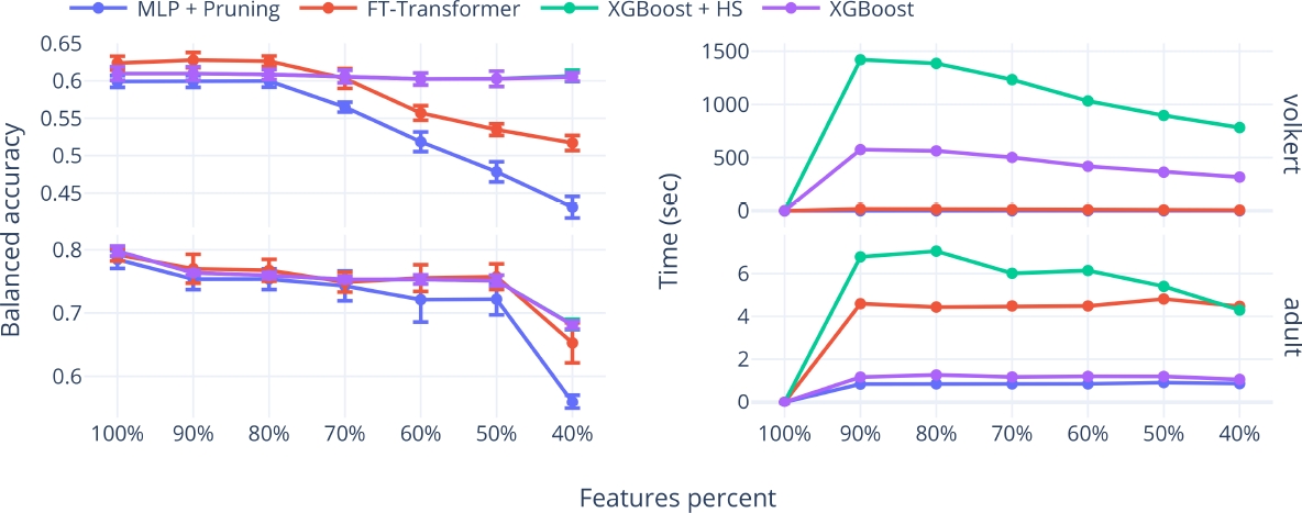
Fig. 1
Mean and standard deviation of cross-validation balanced accuracy for the best-performing architecture in each approach (left) and the elapsed time required to determine the balanced accuracies shown on the left (right), for the volkert and adult datasets
Mean and standard deviation of cross-validation balanced accuracy for the best-performing architecture in each approach (left) and the elapsed time required to determine the balanced accuracies shown on the left (right), for the volkert and adult datasets
The plots include the mean and standard deviations of the cross-validation balanced accuracy against the time required to obtain the balanced accuracies for each evaluation method when using the decision-tree-based feature selection algorithm.
As will be shown in Section 5.3, the decision-tree-based algorithm was the best method for reducing the number of features. The volkert dataset demonstrates a case where the proposed methods excel in efficiency, requiring significantly less time compared to methods that require retraining. However, the effectiveness is only maintained when the removal of low-relevance features is up to 20%.
Conversely, in the adult dataset, the required time for the FT-Transformer, even without retraining, is higher than the time required for XGBoost. Regarding the balanced accuracy degradation, both methods achieve similar results.
The adult dataset represents a poor case for the application of the proposed methods. Figure 2 presents the cross-validation balanced accuracies and the required time for the other datasets. Across all datasets, the time needed to evaluate the low-relevance feature removals is lower than the time required for methods that need retraining.
Thumbnail
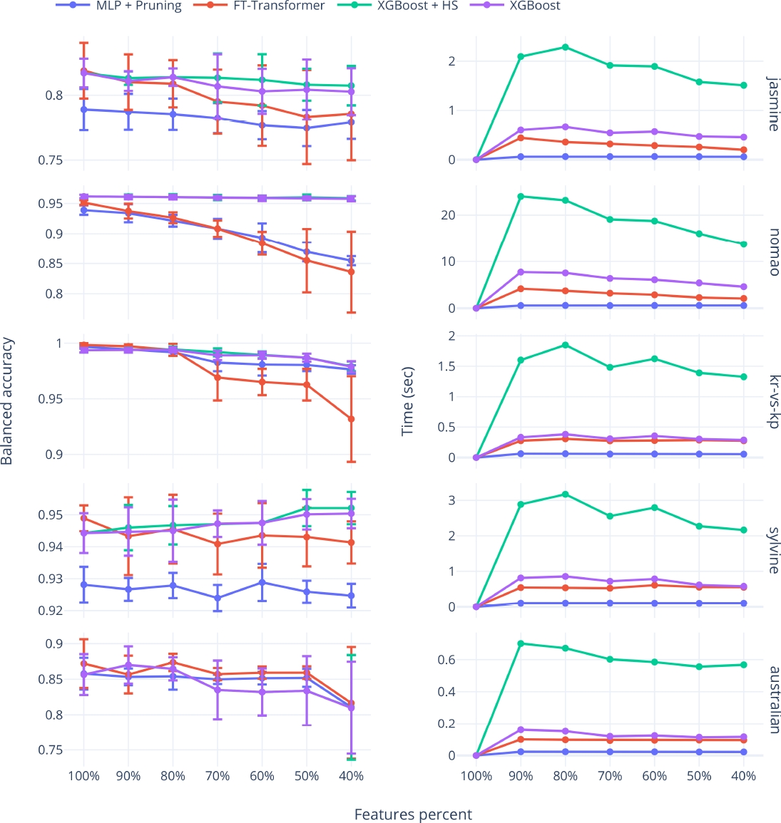
Fig. 2
Mean and standard deviation of cross-validation balanced accuracy for the best-performing architecture in each approach (left) and the elapsed time required to determine the balanced accuracies shown on the left (right), for the jasmine, nomao, kr-vs-kp, sylvine, and australian datasets
Mean and standard deviation of cross-validation balanced accuracy for the best-performing architecture in each approach (left) and the elapsed time required to determine the balanced accuracies shown on the left (right), for the jasmine, nomao, kr-vs-kp, sylvine, and australian datasets
Notably, for every dataset, the degradation in the balanced accuracy of at least one of the proposed methods is very similar to the methods requiring retraining, when the number of selected features ranges between 100% and 80%.
Table 4 shows the balanced accuracies in the test set when using 80% of the features. These results are comparable to those presented in Table 3. The key observation is that for every dataset, the results of every method remain competitive, and even for the volkert, jasmine, sylvine, and australian datasets, the balanced accuracy is higher when using a lower number of features. This highlights the importance of performing feature selection for removing redundant or noisy variables.
Table 4
Test balanced accuracy for each considered method when training using the 80% of the features selected using the decision-tree-based algorithm
Test balanced accuracy for each considered method when training using the 80% of the features selected using the decision-tree-based algorithm
| Dataset | FT-Transformer | MLP + Pruning | XGBoost | XGBoost + HS |
| volkert | 63.611 | 60.178 | 60.126 | 60.126 |
| jasmine | 80.606 | 77.602 | 80.848 | 80.848 |
| nomao | 94.189 | 94.639 | 96.320 | 96.215 |
| kr-vs-kp | 99.369 | 98.429 | 97.190 | 99.687 |
| sylvine | 93.931 | 93.051 | 95.370 | 95.466 |
| australian | 87.428 | 82.063 | 89.067 | 89.067 |
| adult | 75.731 | 74.390 | 73.676 | 73.676 |
To quantify and summarize the observed performance results, we computed the degradation percentage with respect to the balanced accuracy achieved when using 100% of the features for a specific dataset and every method. Given a specific dataset
e4d ( D , ℋ , ℱ ) = [ 1 − max h ∈ ℋ ℬ ( D ℱ , h ) max h ∈ ℋ ℬ ( D , h ) ] ⋅ 100 ,
where
Table 5 shows the mean and standard deviation of the degradation percentages, averaged across all subsets of features generated, ranging from 100% to 40% for each dataset.
Table 5
Mean degradation percentages for each dataset, considering features percentages ranging from 100% to 40%
Mean degradation percentages for each dataset, considering features percentages ranging from 100% to 40%
| Dataset | FT-Transformer | MLP | XGBoost + HS | XGBoost |
| volkert | ||||
| jasmine | ||||
| nomao | ||||
| kr-vs-kp | ||||
| sylvine | ||||
| australian | ||||
| adult |
Negative degradations indicate an improvement over the models trained with the entire feature set. As expected, the highest degradation percentages correspond to methods that were not retrained.
However, the mean degradation percentage for the proposed methods remains below 10%. In contrast to the degradation, the models that do not require retraining exhibit significantly shorter required times.
To compare and summarize the required time for each method, we considered the ratio between every method and the fastest method, which is the MLP approach. Let
e5s ( D ℱ , ℋ ) = T ( D ℱ , ℋ ) T ( D ℱ , ℋ M L P ) .
Table 6 presents the minimum and maximum speed ratios of all subsets of features generated, ranging from 100% to 40% for each dataset. As observed, the FT-Transformer is generally the fastest method, excluding the MLP approach, while the XGBoost + HS is the slowest. Even when the XGBoost + HS is the correct way to perform the tests, the XGBoost was a heuristic method that could work but invested less time.
Table 6
Speed ratios for each approach and dataset, considering feature percentages from 100% to 40%. The MLP was omitted since it was the base for the comparison
Speed ratios for each approach and dataset, considering feature percentages from 100% to 40%. The MLP was omitted since it was the base for the comparison
| Dataset | FT-Transformer | XGBoost + HS | XGBoost |
| volkert | |||
| jasmine | |||
| nomao | |||
| kr-vs-kp | |||
| sylvine | |||
| australian | |||
| adult |
In this case, the proposed methods outperform the efficiency, showing to be up to 300 times faster. It is important to note that the speed ratios of these approaches are closer when using small datasets. However, as the number of instances and features increases, the difference in speed ratios becomes more significant.
5.3 Feature Selection Algorithms Performance
To determine the best feature selection algorithm, we analyze the distributions of the degradation percentages for each feature selection algorithm. Figure 3 shows the distribution of the degradation ratio, computed as in Equation 4, for each feature selection algorithm and percentage of features selected, across all datasets.
Thumbnail
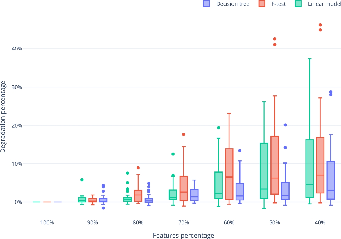
Fig. 3
Percentage of features selected versus the degradation ratio for each algorithm used for feature selection
Percentage of features selected versus the degradation ratio for each algorithm used for feature selection
As observed, the decision tree algorithm generally shows the lowest degradation median and the smallest interquartile range. This indicates that the concentration of the degradations tends to be the smallest among all feature selection algorithms considered, making it the most suitable option for feature removal.
6 Conclusions
In this study, we have evaluated the impact of removing low-relevance features using non-retrained networks. To select low-relevant features, we employed three feature selection algorithms: The embedded decision tree, the F-test, and the embedded linear model. To avoid the retraining procedure, we proposed the use of two architectures: a pruned MLP and the FT-Transformer, leveraging their abilities to create predictions even when certain features are removed.
Our results demonstrate the viability of this approach. When removing up to 60% of low-relevance features, we achieved performance degradations lower than 10%. Crucially, by avoiding retraining, we were able to speed up the decision-making process by up to 300 times, especially for large datasets.
Moreover, we found that using up to 20% of the low-relevant features, the non-retrained neural networks could be employed as final predictive models without sacrificing significant performance compared to retraining-based methods. This last finding is particularly noteworthy.
When working with large datasets, the high costs associated with retraining models as features are removed can be prohibitive. However, by leveraging our proposed non-retrained techniques, these expenses can be largely avoided.
Furthermore, our analysis of the degradation distributions revealed that the embedded decision-tree-based feature selection algorithm outperformed both linear model coefficients and the F-test in identifying the most appropriate low-relevant features to remove.
Acknowledgments
Uriel Corona-Bermúdez and Erendira Corona-Bermúdez thanks CONAHCyT for the scholarship granted towards pursuing his graduate studies.
References
- 1. Ba, J. L., Kiros, J. R., Hinton, G. E. (2016). Layer normalization. arXiv. DOI: 10.48550/arxiv.1607.06450. Links
- 2. Bee-Wah, Y., Ibrahim, N., Abdul-Hamid, H., Abdul-Rahman, S., Simon, F. (2018). Feature selection methods: Case of filter and wrapper approaches for maximising classification accuracy. Pertanika Journal of Science and Technology, Vol. 26, No. 1, pp. 329–340. Links
- 3. Casalicchio, G., Bossek, J., Lang, M., Kirchhoff, D., Kerschke, P., Hofner, B., Seibold, H., Vanschoren, J., Bischl, B. (2017). OpenML: An R package to connect to the machine learning platform OpenML. Computational Statistics, Vol. 34, No. 3, pp. 977–991. DOI: 10.1007/s00180-017-0742-2. Links
- 4. Chen, T., Guestrin, C. (2016). XGBoost: A scalable tree boosting system. Proceedings of the 22nd Association for Computing Machinery’s Special Interest Group on Knowledge Discovery and Data Mining International Conference on Knowledge Discovery and Data Mining, Association for Computing Machinery, pp. 785–794. DOI: 10.1145/2939672.2939785. Links
- 5. Devlin, J., Chang, M. W., Lee, K., Toutanova, K. (2018). BERT: Pre-training of deep bidirectional transformers for language understanding. Proceedings of the Conference of the North American Chapter of the Association for Computational Linguistics: Human Language Technologies, Vol. 1, pp. 4171–4186. DOI: 10.18653/v1/n19-1423. Links
- 6. Ghosh, M., Guha, R., Sarkar, R., Abraham, A. (2019). A wrapper-filter feature selection technique based on ant colony optimization. Neural Computing and Applications, Vol. 32, No. 12, pp. 7839–7857. DOI: 10.1007/s00521-019-04171-3. Links
- 7. Gorishniy, Y., Rubachev, I., Khrulkov, V., Babenko, A. (2021). Revisiting deep learning models for tabular data. 35th Conference on Neural Information Processing System, pp. 1–25. DOI: 10.48550/arXiv.2106.11959. Links
- 8. Guyon, I., Elisseeff, A. (2003). An introduction of variable and feature selection. The Journal of Machine Learning Research, Vol. 3, pp. 1157–1182. Links
- 9. Ho, T. K. (1995). Random decision forests. Proceedings of 3rd International Conference on Document Analysis and Recognition, Vol. 1, pp. 278–282. DOI: 10.1109/ICDAR.1995.598994. Links
- 10. Hollmann, N., Müller, S., Eggensperger, K., Hutter, F. (2022). TabPFN: A transformer that solves small tabular classification problems in a second. International Conference on Learning Representations, pp. 1–37. DOI: 10.48550/arXiv.2207.01848. Links
- 11. Huang, X., Khetan, A., Cvitkovic, M., Karnin, Z. (2020). TabTransformer: Tabular data modeling using contextual embeddings. arXiv. DOI: 10.48550/ARXIV.2012.06678. Links
- 12. Inza, I., Larrañaga, P., Blanco, R., Cerrolaza, A. J. (2004). Filter versus wrapper gene selection approaches in DNA microarray domains. Artificial Intelligence in Medicine, Vol. 31, No. 2, pp. 91–103. DOI: 10.1016/j.artmed.2004.01.007. Links
- 13. Kadra, A., Lindauer, M., Hutter, F., Grabocka, J. (2021). Well-tuned simple nets excel on tabular datasets. 35th Conference on Neural Information Processing Systems, pp. 1–14. Links
- 14. Kuhn, M., Johnson, K. (2013). Applied Predictive Modeling. Springer New York. DOI: 10.1007/978-1-4614-6849-3. Links
- 15. Morey, T. (2015). Customer data: Designing for transparency and trust. Harvard Business Review, Vol. May. 2015, pp. 96–105. Links
- 16. Pedregosa, F., Varoquaux, G., Gramfort, A., Michel, V., Thirion, B., Grisel, O., Blondel, M., Prettenhofer, P., Weiss, R., Dubourg, V., Vanderplas, J., Passos, A., Cournapeau, D., Brucher, M., Perrot, M., Duchesnay, E. (2011). Scikit-learn: Machine learning in Python. Journal of Machine Learning Research, Vol. 12, No. 85, pp. 2825–2830. Links
- 17. Pudjihartono, N., Fadason, T., Kempa-Liehr, A. W., O’Sullivan, J. M. (2022). A review of feature selection methods for machine learning-based disease risk prediction. Frontiers in Bioinformatics, Vol. 2. DOI: 10.3389/fbinf.2022.927312. Links
- 18. Russell, S., Norvig, P. (2010). Artificial Intelligence: A Modern Approach. Prentice Hall. Links
- 19. Vaswani, A., Shazeer, N., Parmar, N., Uszkoreit, J., Jones, L., Gomez, A. N., Kaiser, Ł., Polosukhin, I. (2017). Attention is all you need. Advances in Neural Information Processing Systems, Vol. 30. Links
- 20. Venkat, N. (2018). The curse of dimensionality: Inside out. DOI: 10.13140/RG.2.2.29631.36006. Links
- 21. Wang, Q., Li, B., Xiao, T., Zhu, J., Li, C., Wong, D. F., Chao, L. S. (2019). Learning deep transformer models for machine translation. Proceedings of the 57th Annual Meeting of the Association for Computational Linguistics, pp. 1810–1822. DOI: 10.48550/ARXIV.1906.01787. Links
- 22. Wooldridge, J. M. (2013). Introductory econometrics: A modern approach. South-Western. Links
- 23. Zhang, C., Ma, Y. (2012). Ensemble machine learning: Methods and applications. Springer Publishing Company, Incorporated. Links