Thermodynamics and statistical physics
Landau levels for a Weyl pair in a monolayer medium and thermal quantities

-
Publication dates-
February 24, 2025
Nov-Dec , 2023
- Article in PDF
- Article in XML
- Automatic translation
- Send this article by e-mail
- Share this article +
Abstract
In this paper, we consider a Weyl pair under the effect of an external uniform magnetic field in a monolayer medium without considering any charge-charge interaction between the particles. Choosing the interaction of the particles with the magnetic field in the symmetric gauge we seek for an analytical solution of the corresponding form of a one-time fully-covariant two-body Dirac equation derived from quantum electrodynamics via the action principle. As it is usual with two-body problems, we separate the relative motion and center of mass motion coordinates. Assuming the center of mass is at rest, we derive a matrix equation in terms of the relative motion coordinates without considering any group theoretical method. This equation gives a wave equation in exactly soluble form and accordingly we obtain the spinor components and complete energy eigen-states (in closed form) for such a spinless composite structure. Our results not only give exact Landau levels for such a Weyl pair in a monolayer medium but also show the considered system behaves as a two-dimensional harmonic oscillator. Furthermore, our findings give exactly the excited states of a Weyl particle under the effect of uniform external magnetic field in a monolayer graphene sheet and there is no imprint to distinguish these modes from each other. This means that the performed experiments based on Landau levels for a monolayer graphene sheet may actually involve many-body effects. Our results provide a suitable basis to analyze the associated thermal quantities and accordingly we discuss the thermal properties by determining free energy, total energy, entropy and specific heat for the composite system in question.
Keywords::
Landau levels, graphene, Weyl fermions, charge carriers, many-body system, thermal properties
1. Introduction
In the non-relativistic quantum mechanics frame, the dynamics of two-body systems is investigated through one-time equations including inter-particle interaction potentials depending on relative radial coordinate and this is the wellknown way to describe the bound states, resonance states as well as the scattering states. These equations include, of course, two-body wave functions. Relativistic quantum mechanics, phenomenologically establishes two-body equations to analyse the dynamics of two interacting particles and these equations consist of free Hamiltonians for each particle besides inter-particle interaction potentials. Even though, one of the main problems is how to choose the interaction potentials, which are chosen phenomenologically. That is, mesonic or electrodynamic (one-boson or one-photon exchange) potentials are preferred in general. Also, two-time problem appears in these phenomenologically constructed two-body equations because each particle feels its proper time. After the Dirac equation was written, the first acceptable attempt to write a two-body Dirac equation was made by Breit [1]. This equation includes two free Dirac Hamiltonians plus an interaction term established by modifying the Darwin potential. However, this equation works properly only in the weak coupling regime due to the retardation effects. That is, it cannot give precise results if the particles have high velocities or the interaction is large range. This was a serious problem that must be overcome. To overcome that another formalism was introduced by Bethe and Salpeter by starting from the Quantum Field Theory [2]. However, this new formalism could only provide approximate solutions for bound states due to the relative time difference between particles. Thus, the required equation including relativistic kinematics had to be exactly soluble in 3+1 dimensions and had to be a one-time fully-covariant two-body equation taking into account the retardation effects and including correct spin algebra. Furthermore, such an equation had to be usable in curved spaces. In Ref. [3], Barut has shown us how it is possible to derive a complete and one time fully-covariant two-body Dirac equation from Quantum Electrodynamics. This equation includes the correct spin algebra spanned by direct (Kronecker) product of Dirac matrices, takes into account the retardation effects, includes the most general electric and magnetic potentials [3] and moreover it can be usable in curved spaces [4]. In 3+1 dimensions, the solution of the Barut’s equation requires group theoretical methods to separate radial and angular parts. Briefly, this equation leads to 16 equations and these equations can be reduced into 8 equations thanks to symmetry. However, it results in two second-order differential equations (coupled) or four first-order equations. This means that the solution of this equation for Hydrogen-like systems could be obtained only through a perturbative way [6] and related precise solutions cannot be obtained. In 3+1 dimensions, Moshinsky and Loyola used the Barut’s equation to analyze a Dirac pair with Dirac oscillator interaction and applied the obtained perturbative results to estimate mass spectra for composite particles such as mesons and baryons [7].
-
1The effect of retardation on the interaction of two electronsPhysical Review, 1929
-
2A relativistic equation for bound-state problemsPhysical Review, 1951
-
3Derivation of Nonperturbative Relativistic Two-Body Equations from the Action Principle in QuantumelectrodynamicsFortschritte der Physik/Progress of Physics, 1985
-
3Derivation of Nonperturbative Relativistic Two-Body Equations from the Action Principle in QuantumelectrodynamicsFortschritte der Physik/Progress of Physics, 1985
-
4An interacting fermion-antifermion pair in the spacetime background generated by static cosmic stringPhysics Letters B, 2020
-
6A new approach to bound-state quan-¨ tum electrodynamics: I. TheoryPhysica A: Statistical Mechanics and its Applications, 1987
-
7Barut equation for the particleantiparticle system with a Dirac oscillator interactionFoundations of physics, 1993
In 2+1 dimensions, relativistic quantum theory and gravity have gained interest after the seminal papers in the Refs. [8,9] and discovery of the Banados-Teitelboim-Zanelli black hole [10] and Graphene [11, 35]. Prior to the aforementioned discoveries, it was believed that 2+1 dimensional studies can be useful only for discussing some conceptual issues. Graphene is a two-dimensional (2D) material exhibiting exceptionally high crystal and very high electronic quality [11,35]. This 2D material is formed by carbon atoms in a honeycomb lattice. Low energy electronic spectrum of the graphene can be described by massless Dirac particles (electron and hole) called as Weyl fermions. Graphene and 2D materials are the premier sources of the latest information on commercial and practical applications of 2D materials. These materials are defined as crystalline materials consisting of single or few-layer atoms, in which the inter-atomic interactions are much stronger than those along the stacking direction. They have unique physical and chemical properties due to their reduced dimensionality and quantum confinement effects [36, 37]. These properties enable particles or quasiparticles such as electrons, excitons and magnons to exhibit exotic behaviors differing from their 3D bulk counterparts stemming from the quantum confinement effect. They have attracted tremendous research interest in recent years because of their potential applications in various fields, such as nanoelectronics, optoelectronics, the quantum Hall effect, phase space representation of Wigner functions, quantum heat engine and excitonic systems (see the following Refs. [38-46]). Thus, investigations based on the dynamics of a Weyl pair exposed to an external magnetic field in a monolayer medium can be very useful for clarifying some points. To do this, the fully-covariant two-body Dirac equation can be very useful to determine precise solutions.
-
8Three-dimensional Einstein gravity: dynamics of flat spaceAnnals of Physics, 1984
-
92+1 dimensional gravity as an exactly soluble systemNuclear Physics B, 1988
-
10Black hole in threedimensional spacetimePhysical Review Letters, 1992
-
11Electric field effect in atomically thin carbon filmsScience, 2004
-
35Quantum field theory in a magnetic field: From quantum chromodynamics to graphene and Dirac semimetalsPhysics Reports, 2015
-
11Electric field effect in atomically thin carbon filmsScience, 2004
-
35Quantum field theory in a magnetic field: From quantum chromodynamics to graphene and Dirac semimetalsPhysics Reports, 2015
-
36Recent Advances for the Synthesis and Applications of 2-Dimensional Ternary Layered MaterialsResearch, 2023
-
37Neto, 2D materials and van der Waals heterostructuresScience, 2016
-
38Novel electric field effects on Landau levels in graphenePhysical Review Letters, 2007
-
46Evolution of Landau levels into edge states in grapheneNature Communications, 2013
In this paper, we consider a Weyl pair under the effect of an external uniform magnetic field in a homogeneous monolayer medium and try to determine the dynamics of such a pair by solving the corresponding form of the fully-covariant two-body Dirac equation. To do this, we choose the coupling
of each particle with the external field in the symmetric gauge which allows us to compare the result with the related relativistic oscillators and arrive at a wave equation for such a spinless static system. We obtain energy eigen-states besides the associated spinor components and then we discuss the results in detail. The form of the obtained non-perturbative energy spectrum allows us to determine the associated thermal quantities and we also discuss the thermal properties by determining free energy, total energy, entropy and specific heat for the system in question.
2. Two-body Dirac equation
In this part, we will introduce the covariant two-body equation and will be interested in the relative motion of a mutually non-interacting fermion-antifermion pair exposed to an external uniform magnetic field, by choosing the interaction of the particles with the external field in symmetric gauge, so that we can obtain precise solutions. Then, for the system in question, we will derive the corresponding form of the covariant two-body Dirac equation and will arrive at a set of coupled equations in matrix form. Here, it is worth mentioning that choosing this gauge allows us also to write the equations in the most symmetric form. The generalized form of this equation can be written as [3-5]
-
3Derivation of Nonperturbative Relativistic Two-Body Equations from the Action Principle in QuantumelectrodynamicsFortschritte der Physik/Progress of Physics, 1985
-
5Exact solution for a fermion-antifermion system with Cornell type nonminimal coupling in the topological defect-generated spacetimePhysics of the Dark Universe, 2022
in which f and
-
14Exact solution of Dirac equation in 2+1¨ dimensional gravityJournal of mathematical physics, 2007
-
14Exact solution of Dirac equation in 2+1¨ dimensional gravityJournal of mathematical physics, 2007
-
15Dynamics of a composite system in a point source-induced space-timeInternational Journal of modern Physics A, 2021
-
16Dirac oscillator in an external magnetic fieldPhysics Letters A, 2010
-
13Electronic properties of graphene in a strong magnetic fieldReviews of Modern Physics, 2011
-
17Exact solution of an exciton energy for a monolayer mediumScientific reports, 2019
which leads
and
ii
-
18Relativistic Landau levels for a fermionantifermion pair interacting through Dirac oscillator interactionThe European Physical Journal C, 2021
-
17Exact solution of an exciton energy for a monolayer mediumScientific reports, 2019
in which the dot means derivative with respect to the r, for a static spinless composite system consisting of a Weyl (m = 0) pair exposed to an external uniform magnetic field in a spatially flat monolayer medium if
and only if E ≠ 0. That is ϑ2(r) = 0 if one considers the E ≠ 0 case. This cannot appear when m ≠ 0, of course.
3. Landau levels for a Weyl pair
Here, we try to determine exact Landau levels for a static Weyl pair under the
influence of an external uniform magnetic field in a flat monolayer medium. To
acquire this, we look for an analytical solution of the set of equations in Eq. (3).
For this purpose, we start by considering a dimension less independent variable,
ξ = Br
2 which leads
one of which is algebraic. In the second and third equation, we can easily see that the ϑ3(ξ) and ϑ4(ξ) components can be expressed in terms of ϑ1(ξ). That is the first equation in Eq. (4) gives a wave equation for the component ϑ1(ξ) and this wave equation can be rewritten by considering an ansatz function, ϑ1(ξ) = ϑ(ξ) √ξ, as
Solution function of this equation can be expressed in terms of the Kummer Confluent
Hypergeometric function [19,20]
-
19Mathematical Methods for Physicists, 2012
-
20Relativistic vector bosons with non-minimal coupling in the spinning cosmic string spacetimeFew-Body Systems, 2021
-
21Handbook of Mathematical Functions, 1965
This function is divergent when
where
-
22Quantum field theory in a magnetic field: From quantum chromodynamics to graphene and Dirac semimetalsPhysics Reports, 2015
From (6), we see that the energy of such a static pair depends on the Fermi velocity
(V ∼ c/300 [13]), reduced
Planck constant
-
13Electronic properties of graphene in a strong magnetic fieldReviews of Modern Physics, 2011
Thumbnail
![Dependence of the energy levels on the amplitude of the external
uniform magnetic field (see also [25]).](/img/revistas/rmf/v69n6//0035-001X-rmf-69-06-e61701-gf1.jpg)
FIGURE 1
Dependence of the energy levels on the amplitude of the external uniform magnetic field (see also [25]).
Dependence of the energy levels on the amplitude of the external uniform magnetic field (see also [25]).
4. Thermal properties
4.1. Euler-Maclaurin formula
In this section, we calculate the different thermodynamic variables using the standard definition of the partition function Z. In order to obtain more accurate quantities, we shall use the infinite sums of n-contributions of the energy multiplied by the constant β. Therefore, it is convenient to write the different thermodynamic variables in terms of these sums and perform a numerical computation for each variable for a certain range of the temperature T. The partition function is given by
here β = 1/kT, k is the Boltzmann constant. Here, considering only positive energies in calculating, the partition function can be justified as follows: (i) The Dirac equation has an exact Foldy-Wouthuysen transformation and this means that positive and negative energy solutions do not mix. (ii) We assume that the negative energy (antiparticle) as fully occupied: It is correct because all fermions are ordered by the Pauli’s principle. Now, to evaluate the partition function, we use the Euler-Maclaurin formula which gives the difference between an integral and a closely related sum. It makes the connection between the sum and the integral explicit for sufficiently smooth functions. In the most general form, it can be written as [26,27]
-
26Special Functions, 1999
-
27Quantum Calculus, 2001
where α and b are arbitrary real numbers with difference b−α being a positive integer number, B n and b n are Bernoulli polynomials and numbers, respectively, and k is any positive integer. The condition we impose on the real function f is that it should have continuous k-th derivative. The symbol {x} for a real number x denotes the fractional part of x. Here, the remainder term (error term)
is the most essential in the Euler-Maclaurin equation. If f (x) and all its derivatives tend to 0 as x → ∞, the formula can be simplified:
The first several Bernoulli numbers are the following:
The odd terms in the sequence are all 0 except the first one b 1. The Bernoulli polynomials B n can be defined by a generating function
The first few Bernoulli polynomials are:
Also, more general, for a positive integer n, we define the
periodic Bernoullian function
-
28The fractional parts of the Bernoulli numbersIllinois Journal of Mathematics, 1980
-
29The Euler-Maclaurin formula revisitedJournal of the Australian Mathematical Society: Series B, Applied Mathematics, 1998
In what follows, all thermodynamic properties of the system in question, such as
the free energy, the entropy, total energy and the specific heat, can be
obtained through the numerical partition function Z. Looking
for simplicity, we will prefer to use the natural units
4.2. Numerical results and discussions
Now, we discuss and comment on our numerical results on the calculation of the thermal quantities obtained via the partition function. We should mention that, in all the figures, we have used adimensional quantities. According to the above considerations, we can define the thermodynamic functions of interest as follows:
and
The integral appearing in (11) can be calculate as follows:
After fixed k = 4, the explicit form of the partition function (Eq. (15)) is given by
With the aid of the partition function Z the thermal properties
of the considered system can be found easily. These thermodynamic functions are
represented according to the inverse temperature β and for
different values of the magnetic field B. Thus, we have chosen
B =
1,5,10,15,20,25,30.
The dimensionless variable
-
30The thermal properties of a two-dimensional Dirac oscillator under an external magnetic fieldThe European Physical Journal Plus, 2013
This temperature is similar to the Debye temperature in the solid state [30-32]. It also depends inversely on the intensity of the magnet field. Table II provides some values for this temperature in SI for the case of graphene. One has massless particles moving through the honeycomb lattice with a velocity V = 1.1 × 10⁶ m/s the so-called Fermi velocity [31,33].
-
30The thermal properties of a two-dimensional Dirac oscillator under an external magnetic fieldThe European Physical Journal Plus, 2013
-
32Three-dimensional Dirac oscillator in a thermal bathEurophysics Letters, 2014
-
31Thermodynamic properties of the graphene in a magnetic field via the two-dimensional Dirac oscillatorPhysica Scripta, 2015
-
33Infrared Spectroscopy of Landau Levels of GraphenePhysical Review Letters, 2007
TABLE I
For e = 1, ℏ = 1 and c = 1.
For e = 1, ℏ = 1 and c = 1.
| B0 | lB |
| 1 | 1 |
| 5 | 0.447 |
| 10 | 0.316 |
| 15 | 0.258 |
| 20 | 0.223 |
| 25 | 0.2 |
| 30 | 0.182 |
TABLE II
Some values of the characteristic temperature T0.
Some values of the characteristic temperature T0.
| B(Tesla) | lB (× 10−8 meter) | T0(K) |
| 1 | 2.56 | 655 |
| 5 | 1.14 | 1465 |
| 10 | 0.81 | 2071 |
| 15 | 0.67 | 2537 |
| 20 | 0.58 | 2929 |
| 25 | 0.51 | 3275 |
| 30 | 0.47 | 3587 |
The obtained results are illustrated in the Fig. 2. According to this Figure, the following may be observed:
-
The effect of the magnetic field is observed in all thermal quantities. This dependency is inversely with the field.
-
Entropy and specific heat curves tend to zero at low temperatures.
-
Comparing with the existing studies, this remark is due to the adding the reminder term in the Euler-Mclaurin formula which has been dropped in these studies (see for example [30,34]). This term has the role the avoid the divergence in the partition function and consequently all thermal quantities of our problem.
-
Now, at very high temperatures, the specific heat curves converge to 2. This convergence depends inversely on the applied magnetic field B. The convergence to this point is faster in the lower region of the magnetic field B than in higher values of it.
-
30The thermal properties of a two-dimensional Dirac oscillator under an external magnetic fieldThe European Physical Journal Plus, 2013
-
34One-dimensional thermal properties of the Kemmer oscillatorPhysica Scripta, 2007
Thumbnail
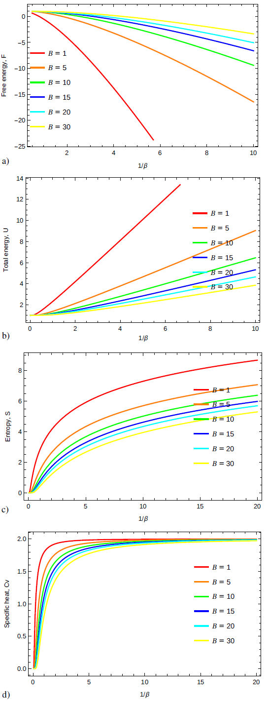
FIGURE 2
Thermal properties as a function of 1/β for different values of the magnetic length l B : a) Free energy F. b) Total energy U. c) Entropy S. d) Specific heat C v .
Thermal properties as a function of 1/β for different values of the magnetic length l B : a) Free energy F. b) Total energy U. c) Entropy S. d) Specific heat C v .
5. Summary and results
In this manuscript, we have studied the dynamics of a Weyl pair (mutually
non-interacting) exposed to an external uniform magnetic field in a monolayer
medium. To do this, we have used the fully-covariant two-body Dirac equation derived
from Quantum Electrodynamics via the action principle. First of all, by choosing the
interaction of the particles with the external uniform magnetic field in the
symmetric gauge, we have written the corresponding form of this onetime two-body
equation for a general fermion-antifermion pair. Afterwards, we have separated the
center of mass motion coordinates and relative motion coordinates as is usual with
two-body problems. By assuming the center of mass is at rest at the spatial origin,
we have arrived at a matrix equation consisting of four first-order equations
(coupled) in terms of the relative motion coordinates. We have transformed the
background into the polar space so that we can exploit the angular symmetry. Then,
we have reduced the obtained matrix equation resulting in three equations, one of
which is algebraic, for a such a spinless composite system formed by a Weyl pair.
These equations allow us to derive a wave equation in exactly soluble form. Solution
function of this equation can be expressed in terms of the Kummer Confluent
Hypergeometric function. Accordingly we have obtained the energy spectrum (see Eq.
(6)) in closed-form besides the defined spinor components (see Eq. (7)). Equation
(6) has shown that energy of such a pair depends on the Fermi velocity (V),
magnitude of the elementary electrical charge (e), amplitude of the
external uniform magnetic field (B0) besides the reduced Planck constant
-
23Dirac electron in graphene with magnetic fields arising from first-order intertwining operatorsJournal of Physics A: Mathematical and Theoretical, 2020
-
13Electronic properties of graphene in a strong magnetic fieldReviews of Modern Physics, 2011
-
24Diamagnetism of graphitePhysical Review, 1956
-
25Observation of Landau levels of Dirac fermions in graphiteNature Physics, 2007
-
The third law of thermodynamics of entropy and specific heat
is well fulfilled.
-
These thermal properties depend inversely with the magnetic field.
-
In higher temperatures, all the curves of specific heat tend towards 2. When the magnetic field increases, this convergence goes towards this limit very slowly.
Funding
There is no funding regarding this research.
Data Availability Statement
No Data associated in the manuscript.
Conflict of Interest Statement
No conflict of interest has been declared by the authors.
References
-
1G. Breit, The effect of retardation on the interaction of two electrons, Physical Review 34 (1929) 553, https://doi.org/10.1103/PhysRev.34.553 Links
-
2E. E. Salpeter, and H. A. Bethe, A relativistic equation for bound-state problems, Physical Review 84 (1951) 1232, https://doi.org/10.1103/PhysRev.84.1232 Links
-
3O. Barut and S. Komy, Derivation of Nonperturbative Relativistic Two-Body Equations from the Action Principle in Quantumelectrodynamics, Fortschritte der Physik/Progress of Physics 33 (1985) 309, https://doi.org/10.1002/prop.2190330602 Links
-
4Guvendi and Y. Sucu, An interacting fermion-antifermion pair in the spacetime background generated by static cosmic string, Physics Letters B 811 (2020) 135960, https://doi.org/10.1016/j.physletb.2020.135960 Links
-
5Guvendi, S. Zare and H. Hassanabadi, Exact solution for a fermion-antifermion system with Cornell type nonminimal coupling in the topological defect-generated spacetime, Physics of the Dark Universe 38 (2022) 101133, https://doi.org/10.1016/j.dark.2022.101133 Links
-
6O. Barut and N. Unal, A new approach to bound-state quan-¨ tum electrodynamics: I. Theory, Physica A: Statistical Mechanics and its Applications 142 (1987) 467, https://doi.org/10.1016/0378-4371(87)90036-7 Links
-
7M. Moshinsky and G. Loyola, Barut equation for the particleantiparticle system with a Dirac oscillator interaction, Foundations of physics 23 (1993) 197, https://doi.org/10.1007/BF01883624 Links
-
8S. Deser, R. Jackiw, and G. Hooft, Three-dimensional Einstein gravity: dynamics of flat space, Annals of Physics 152 (1984) 220, https://doi.org/10.1016/0003-4916(84)90085-X Links
-
9E. Witten, 2+1 dimensional gravity as an exactly soluble system, Nuclear Physics B 311 (1988) 46, https://doi.org/10.1016/0550-3213(88)90143-5 Links
-
10M. Banados, C. Teitelboim and J. Zanelli, Black hole in threedimensional spacetime, Physical Review Letters 69 (1992) 1849, https://doi.org/10.1103/PhysRevLett. 69.1849 Links
-
11K. S. Novoselov et al., Electric field effect in atomically thin carbon films, Science 306 (2004) 666, https://doi.org/10.1126/science.1102896 Links
-
12K. Geim and K. S. Novoselov, The rise of graphene, Nature materials 6 (2007) 183, https://doi.org/10.1038/nmat1849 Links
-
13M. O. Goerbig, Electronic properties of graphene in a strong magnetic field, Reviews of Modern Physics 83 (2011) 1193, https://doi.org/10.1103/RevModPhys.83.1193 Links
-
14Y. Sucu and N. Unal, Exact solution of Dirac equation in 2+1¨ dimensional gravity, Journal of mathematical physics 48 (2007) 052503, https://doi.org/10.1063/1.2735442 Links
-
15Guvendi, Dynamics of a composite system in a point source-induced space-time, International Journal of modern Physics A 36 (2021) 2150144, https://doi.org/10.1142/S0217751X2150144X Links
-
16P. Mandal and S. Verma, Dirac oscillator in an external magnetic field, Physics Letters A 374 (2010) 1021, https://doi.org/10.1016/j.physleta.2009.12.048 Links
-
17Guvendi, R. Sahin, and Y. Sucu, Exact solution of an exciton energy for a monolayer medium, Scientific reports 9 (2019) 1, https://doi.org/10.1038/s41598-019-45478-4 Links
-
18Guvendi, Relativistic Landau levels for a fermionantifermion pair interacting through Dirac oscillator interaction, The European Physical Journal C 81 (2021) 1, https://doi.org/10.1140/epjc/s10052-021-08913-3 Links
-
19G. B. Arfken, H. J. Weber and F. E. Harris, Mathematical Methods for Physicists, Seventh Edition: A Comprehensive Guide, (Academic Press, Cambridge, 2012), https://www.sciencedirect.com/book/9780123846549/mathematical-methods-for-physicists Links
-
20Guvendi and H. Hassanabadi, Relativistic vector bosons with non-minimal coupling in the spinning cosmic string spacetime, Few-Body Systems 62 (2021) 1, https://doi.org/10.1007/s00601-021-01652-x Links
-
21M. Abramowitz and I. A. Stegum, Handbook of Mathematical Functions, (Dover Publications Inc., New York, 1965). Links
-
22V. A. Miransky and I. A. Shovkovy, Quantum field theory in a magnetic field: From quantum chromodynamics to graphene and Dirac semimetals, Physics Reports 576 (2015) 1, https://doi.org/10.1016/j.physrep.2015.02.003 Links
-
23M. Castillo-Celeita and D. J. Fernández, Dirac electron in graphene with magnetic fields arising from first-order intertwining operators, Journal of Physics A: Mathematical and Theoretical 53 (2020) 035302, https://doi.org/10.1088/1751-8121/ab3f40 Links
-
24J. W. McClure, Diamagnetism of graphite, Physical Review 104 (1956) 666, https://doi.org/10.1103/PhysRev.104.666 Links
-
25G. Li and E. Y. Andrei, Observation of Landau levels of Dirac fermions in graphite, Nature Physics 3 (2007) 623, https://doi.org/10.1038/nphys653 Links
-
26G. Andrews, R. Askey, R. Roy, Special Functions, Cambridge University Press, Cambridge, (1999). Links
-
27V. Kac and P. Cheung, Quantum Calculus, Springer, (2001). Links
-
28P. Erdos and S. S. Wagstaff, The fractional parts of the Bernoulli numbers, Illinois Journal of Mathematics 24 (1980) 104, https://doi.org/10.1215/ijm/1256047799 Links
-
29D. Elliot, The Euler-Maclaurin formula revisited, Journal of the Australian Mathematical Society: Series B, Applied Mathematics 40 (1998) E27, https://doi.org/10.21914/anziamj.v40i0.454 Links
-
30Boumali and H. Hassanabadi, The thermal properties of a two-dimensional Dirac oscillator under an external magnetic field, The European Physical Journal Plus 128 (2013) 124, https://doi.org/10.1140/epjp/i2013-13124-y Links
-
31Boumali, Thermodynamic properties of the graphene in a magnetic field via the two-dimensional Dirac oscillator, Physica Scripta 90 (2015) 045702, https://doi.org/10.1088/0031-8949/90/4/045702 Links
-
32M. H. Pacheco, R. V. Maluf, C.A.S. Almeida, and R. R. Landim, Three-dimensional Dirac oscillator in a thermal bath, Europhysics Letters 108 (2014) 10005, https://doi.org/10.1209/0295-5075/108/10005 Links
-
33Z. Jiang et al., Infrared Spectroscopy of Landau Levels of Graphene, Physical Review Letters 98 (2007) 197403, https://doi.org/10.1103/PhysRevLett.98.197403 Links
-
34Boumali, One-dimensional thermal properties of the Kemmer oscillator, Physica Scripta 76 (2007) 669, https://doi.org/10.1088/0031-8949/76/6/014 Links
-
35V. A. Miransky, and I. A. Shovkovy, Quantum field theory in a magnetic field: From quantum chromodynamics to graphene and Dirac semimetals, Physics Reports 576 (2015) 1, https://doi.org/10.1016/j.physrep.2015.02.003. Links
-
36J. Peng, Z. Chen, B. Ding, and H. M. Cheng, Recent Advances for the Synthesis and Applications of 2-Dimensional Ternary Layered Materials, Research 6 (2023) 1, https://doi.org/10.34133/research.0040 Links
-
37K. S. Novoselov, A. Mishchenko, A. Carvalho, and A. H. Castro, Neto, 2D materials and van der Waals heterostructures, Science 353 (2016) 9439, https://doi.org/10.1126/science.aac9439 Links
-
38V. Lukose, R. Shankar, and G. Baskaran, Novel electric field effects on Landau levels in graphene, Physical Review Letters 98 (2007) 116802, https://doi.org/10.1103/PhysRevLett.98.116802 Links
-
39N. Gu, M. Rudner, A. Young, P. Kim, and L. Levitov, Collapse of Landau levels in gated graphene structures, Physical Review Letters 106 (2011) 066601, https://doi.org/10.1103/PhysRevLett.106.066601 Links
-
40F. Guinea, M. I. Katsnelson, and A. K. Geim, Energy gaps and a zero-field quantum Hall effect in graphene by strain engineering Nature Physics 6 (2010) 30, https://doi.org/10.1038/nphys1420 Links
-
41Y. Betancur-Ocampo, E. Diaz-Bautista, and T. Stegmann, Valley-dependent time evolution of coherent electron states in tilted anisotropic Dirac materials, Physical Review B 105 (2022) 045401, https://doi.org/10.1103/PhysRevB.105.045401 Links
-
42G. J. Iafrate, V. N. Sokolov, and J. B. Krieger, Quantum transport and the Wigner distribution function for Bloch electrons in spatially homogeneous electric and magnetic fields, Physical Review B 96 (2017) 144303, https://doi.org/10.1103/PhysRevB.96.144303 Links
-
43E. Liu, J. van Baren, T. Taniguchi, K. Watanabe, Y. C. Chang, and C. H. Lui, Landau-Quantized Excitonic Absorption and Luminescence in a Monolayer Valley Semiconductor, Physical Review Letters 124 (2020) 097401, https://doi.org/10.1103/PhysRevLett.124.097401 Links
-
44F. J. Pena, and E. Munoz, Magnetostrain-driven quantum engine on a graphene flake, Physical Review E 91 (2015) 052152, https://doi.org/10.1103/PhysRevE.91.052152 Links
-
45A. Greshnov, Room-temperature quantum Hall effect in graphene: the role of the two-dimensional nature of phonons, Journal of Physics: Conference Series 568 (2014) 052010, https://doi:10.1088/1742-6596/568/5/052010. Links
-
46G. Li, A. Luican-Mayer, D. Abanin, L. Levitov, and E. Y. Andrei, Evolution of Landau levels into edge states in graphene, Nature Communications 4 (2013) 1744, https://doi:10.1038/ncomms2767 Links