Artículos

 

The Effect of Trade and Foreign Direct Investment on Inequality: Do Governance and Macroeconomic Stability Matter?

 

El efecto del comercio y la inversión extranjera directa en la desigualdad: ¿importan la gobernanza y la estabilidad macroeconómica?

 

Gerardo Angeles-Castro*

 

* Research economist and head of Research and Graduate Studies, Escuela Superior de Economía (ESE), Instituto Politécnico Nacional (IPN). Mexico City. gangeles@ipn.mx

 

Fecha de recepción: 2 de junio de 2008;
Fecha de aceptación: 9 de marzo de 2010.

 

Abstract

Through dynamic panel data techniques and applying the estimated household income inequality data-set (Galbraith and Kum, 2003), this paper is aimed at exploring the effect of economic variables such as trade, foreign direct investment (FDI) and inflation on inequality, under different scenarios of domestic efficiency and over time. Trade benefits income distribution, whereas FDI and inflation increase inequality. The expansion of exports and employment based on the primary sector does not provide distributional effects, not even in low income countries. Those economies associated with macroeconomic stability and a high governance indicator can mitigate the adverse effect of FDI on income distribution, and enhance the benefits of trade. in the longer run, employment in industry, trade and in particular manufactured exports, can exert more distributional effects, while the adverse effect of FDI and inflation decreases.

Keywords: trade, foreign direct investment, inflation, inequality, good governance, panel data.

 

Resumen

A través de técnicas de panel de datos dinámicos y al aplicar la base de datos de estimadores de desigualdad de ingreso por hogares (Galbraith y Kum, 2003), este artículo explora los efectos de variables económicas tales como comercio, inversión extranjera directa (IED) e inflación sobre la desigualdad, en diferentes escenarios de eficiencia doméstica y a lo largo del tiempo. El comercio beneficia la distribución del ingreso, mientras que la IED y la inflación incrementan la desigualdad. El crecimiento de las exportaciones y el empleo basado en el sector primario no genera efectos distributivos, ni siquiera en países de bajo ingreso. Las economías asociadas con estabilidad macroeconómica y un alto indicador de gobernanza, pueden mitigar el efecto adverso de la IED en la distribución del ingreso e incrementar los beneficios del comercio. en el largo plazo, el empleo industrial, el comercio y en particular las exportaciones manufactureras pueden ejercer más efectos distributivos, mientras que el efecto adverso de la IED y la inflación decrece.

Palabras clave: comercio, inversión extranjera directa, inflación, desigualdad, gobernanza, datos de panel.

JEL classification: C23, f59, O15, P51.

 

Introduction

The surge of market-oriented policies, such as deregulation, privatization, liberalization of markets and macroeconomic discipline, undertaken on a global scale since the early 1980s, has created the preconditions for the expansion of trade and the flow of investments across countries. The theoretical support for these economic policies is the standard neoclassical theory, which argues that trade, investment and, in general, the market mechanisms boost growth and facilitate development. This view also holds that an important factor affecting growth and the effectiveness of the market system is the efficient organization of the domestic economy itself (Gilpin, 1987, pp. 265-266).

The implications of this model for income distribution are that high and sustained rates of growth and the expansion of exports foster employment reduce poverty and eventually provide additional resources that facilitate the distribution of income.

Moreover, economic liberalism facilitates the operation of market forces and the adjustment to world prices, which allow resources to be allocated more efficiently. The theoretical formulations explaining this effect are the orthodox principle of comparative advantages and the Stolper-Samuelson theorem. The latter is a neoclassical two-factor model, in which foreign trade increases the use of the cheaper-abundant factor as exports and imports adjust according to the principle of comparative advantages, while the costly scarce factor is used less. This mechanism increases the income of the factor which is relatively most used in the export sector and which is also most abundant. for example, this factor is conventionally assumed to be unskilled labor in developing countries; by the same token, income distribution is expected to improve.

The set of market-oriented policies is a policy prescription often referred to as the Washington Consensus ¹ or first generation reforms (Ortiz, 2003, pp. 14-17). These terms are applied especially in developing countries.

By applying panel data techniques, with observations across countries and over time, this paper is aimed at testing the effect of the economic variables —trade, investment, macroeconomic discipline and employment— that are assumed to improve income distribution.

Over the last few years, leading globalizers and multilateral institutions have induced support for a set of socio-political norms, and have also recognized the need for a stronger governance dimension. They have added institution building, civil society participation, social and human capital formation, safety nets, transparency and accountability, among others, to the original economic norms or first generation policies. The global governance agenda is a response to the financial crises that have hit emerging markets since 1995; the increasing perception that liberalization brings with it inequality and other subsequent forms of resistance to globalization (Higgott, 2000, pp. 131-140).

This set of socio-political norms is usually called the Post Washington Consensus (PWC) or second generation reforms. The PWC is an attempt to socialize and humanize the operation of market forces, and to legitimize global economic liberalization, although there is also a genuine recognition of the importance of tackling issues of fairness and inequality (Edwards, 1999). in this model, the re-empowerment of the state plays a central role for addressing the socioeconomic dislocation that may be generated by global liberalization. Thus, in this context, the understanding of governance is the effective and efficient management of the modern state.

Moreover, from this perspective domestic efficiency and sound and disciplined macroeconomic policies accentuate the benefits of globalization, and are associated with sustainable economic growth and equity over the long-run. in contrast, those countries which do not adopt sound policies and show evidence of pronounced macroeconomic disequilibria are likely to fall behind in relative terms (IMF, 1997, p. 72; Camdessus, 1998, p. xiv; Higgott and Phillips, 2000, p. 363). in this context, the paper also tests the effects of the PWC approach on income distribution. for this purpose we use variables such as general government expenditure to proxy the size of the state, and subsidies and transfers to proxy the social orientation of the state. We also explore the effect of trade and FDI under different scenarios of macroeconomic stability and governance. finally, we test the effect of human capital formation, represented by secondary school enrollment, on income distribution. education is deemed as one of the key elements in the PWC perspective.

We find that the variable on trade exerts a weak benefit on income distribution, but the benefit increases over the longer run; however, the effect is statistically significant only on the samples which comprise countries associated with good governance or macroeconomic stability. The flow of FDI increases inequality under any scenario, but the effect is mitigated in those countries that exhibit domestic efficiency. inflation worsens inequality in those countries with domestic inefficiency, and this variable adversely affects income distribution even in those countries which exhibit good governance, although, in any case, the effect is weak. inflation serves as a proxy for macroeconomic stability because it is shown that it affects inequality through budget deficit and money supply.

Manufactured exports reduce inequality, whereas the expansion of primary exports does not exert benefit on income distribution under any scenario. employment benefits income distribution; however, when we explore the effects of employment by sector we notice that the expansion of employment in industry reduces inequality; in contrast, employment in agriculture is not able to improve income distribution. Consequently, the analysis of exports and employment by sector suggests that emphasis on primary production does not form the basis for redistributional effects. even those countries with some form of domestic inefficiency, which are associated with lower levels of development and also with comparative advantages supported on natural resources and un-skilled labor, do not seem to improve income distribution with the expansion of primary exports. it is also worth noting that manufactured exports and employment in industry can have longer run benefits on income distribution.

As for the set of socio-political norms underlined in the PWC, we find that domestic efficiency can help to reduce the adverse effect of FDI on income distribution, while it can also help to enhance benefits from trade. More-over, a stronger state, social expenditure, and human capital formation are important factors to decrease inequality. These findings suggest that the PWC represents an improvement to mitigate the adverse effects that the operation of markets can exert on income distribution.

The paper is organized as follows: section I analyzes the characteristics of the data-sets on income distribution available in the literature, and selects the appropriate option for this study. it also presents the features of the explanatory variables included in the model. Section II explains the econometric method applied in the analysis. Section III gives results. finally, concluding remarks are provided in section IV.

 

I. The data

I.1. Data on income inequality

One of the features that characterize the available data-sets on income inequality is that the coverage is sparse and varies widely across countries and over time. in the absence of adequate longitudinal data, some studies attempting to assess the trend of inequality worldwide over time draw general conclusions from cross sectional data, so as to try to overcome this major drawback (Milanovic, 1995; Jha, 1996). However, this type of data does not deal with intertemporal relationships. in addition, other studies restrict attention to a subset of the data, such as five-year intervals (de Gregorio and Lee, 2002; dollar and Kraay, 2004) or group the data in five-year or ten-year averages (deininger and Squire, 1998; Calderón and Chong, 2001), but in these cases there is a risk of bias in the selection of the subset or in the construction of the average, respectively. finally, in order to improve coverage across space and through time, other studies use data-sets measuring a component of overall income inequality (Galbraith and Kum, 2002); however, these data-sets are not representative samples covering all the population.

So as to provide an accurate assessment, the data-set on income inequality must contain a substantial coverage across countries and over time. it must also be consistent and harmonized, and based on a representative measure covering all of the population.

The competing options available in the literature have the following characteristics: the World Bank data-set by deininger and Squire (hereafter, D & S) in its 1996 version and the World income inequality database by UNU/WIDER (2007) are important compilations of Gini coefficients reported in the literature; however, they suffer from a substantial degree of heterogeneity and sparse coverage. The Luxembourg income Study (2007) assembles observations that are more harmonized than the previous two data-sets, since it obtains information from standardized macro-level data, but its coverage is constrained to 29 countries. The UTIP -UINIDO data-set by UTIP (2002) calculates industrial pay-inequality. it has a large coverage and shows evidence of consistency and accuracy, but it is not an index of overall inequality.

The estimated Household income inequality (EHII), constructed by Galbraith and Kum (2003), aims to fill the gaps and correct what they consider errors in the D & S data-set. This indicator takes advantage of the information in D & S and in the UTIP–UNIDO database. As a matter of fact, they replicate the coverage of the latter with estimated measures of household income inequality, taking into account the relationship between industrial pay inequality, household income inequality and an additional set of variables.

Galbraith and Kum (2003, p. 9) underline two advantages of their data-set:

first, the coverage basically matches that of the UTIP–UNIDO exercise, providing substantially annual estimates of household income inequality for most countries, including developing countries that are badly under-represented in D & S. Second, the data set borrows accuracy from the UTIP–UNIDO .. with due adjustment for the different weight of manufacturing in different economies. At the same time, unexplained variations in the D & S income inequality measures are treated as what they probably are: inexplicable. They are therefore disregarded in the calculations of the UTIP Gini coefficients.

The EHII data-set provides consistency, representation of household income inequality, and large coverage; therefore, it can provide further insights for the study of income distribution. As a consequence, we select it from the competing data-sets as a source of information for this study. The major drawback of the data-set is that its most updated period is 1999; nevertheless, the time span is enough to explore long-run effects of the variables involved in the analysis.

I.2. Explanatory variables

The variable for trade is "trade volume", which is the sum of exports and imports of goods and services measured as a share of GDP. Alternatively, we also use "changes in trade volume". So as to test the effect of exports by sector on income distribution, we apply two variables representing the percentage of manufactured exports and the percentage of primary exports to merchandise exports. The source of the variables for trade is the World development indicators (hereafter, WDI) by the World Bank (2007a).

In order to represent the international flow of investment, we use FDI inflow measured as a percentage of GDP; the source of the variable for FDI is a compilation of data from the WDI and UNCTAD (2007).

Geographical and socio-economic factors can cause an unequal flow of FDI across countries and regions. in this respect, Redding and Venables (2004) argue that firms can be reluctant to move production to low wage and unskilled locations, as they prefer areas with better access to markets and supply sources, and show that these geographical characteristics and the way they influence the mobility of firms and plants contribute to explain cross-country variations in per capita income. Ma (2006) shows that the distance of foreign-owned firms from access to international markets and from suppliers of intermediate inputs are important to determine wage inequality across regions in China. in addition, firms can prefer to move production to regions with better infrastructure and more supply of skilled labor, and therefore are likely to increase regional inequality within and between countries. furthermore, some authors have illustrated that FDI with relatively skill-biased technology increases the wage gap of host countries (Wu, 2001).

So as to test if FDI has an effect on inequality through factors such as geographical location, level of wages or income, and skill supply, three additional variables are included in the analysis. firstly, skill supply is represented by gross secondary school enrollment; this indicator is a compilation of data from UNESCO (2007) and WDI. Secondly, a variable on the distance (km) from the capital of each country to any of the three major Cities —New York, Tokyo and London— is introduced to proxy geographical location; the information is taken from the distance calculator (2009). finally, GDP per capita (constant 2000 US dollars) is introduced in the analysis as a proxy of income level; the source is WDI.

Inflation is included as a proxy of macroeconomic mismanagement. it reflects the annual percentage of change in consumer prices, and is taken from the WDI. This analysis also uses standard deviation of inflation for the period 1980-1998, calculated from the same source to construct two sub-samples. The first sub-sample comprises countries with standard deviation lower than 8.5, whereas the second sub-sample groups the countries with standard deviation greater than 8.5. This indicator allows us to assess the effect of economic liberalization on inequality in two different scenarios of macroeconomic stability. The sub-sample classification is carried out through K-means cluster analysis.²

In order to test whether inflation is the result of macroeconomic disequilibrium, a proxy of money supply —money and quasi money (M2) annual growth— and a proxy of budget deficit —government expenditure minus tax revenue as a percentage of GDP— are added to the analysis. The information is calculated with data from WDI. After including these variables the number of observations drops, and, because of constraints on data availability, the exercise is conducted only for the overall sample.

The variables on governance comprise human capital formation, which is one of the main elements included in the concept of governance, and is represented by gross secondary school enrollment. The analysis also includes an aggregate governance indicator by the World Bank (2007b) for the year 1996. it is the average of six indicators measuring the following dimensions of governance: voice and accountability, political stability and absence of violence, government effectiveness, regulatory quality, rule of law, and control of corruption. its score lies between -3.0 and 3.0, with a higher score corresponding to better governance. The indicator is used to construct low governance and high governance sub-samples that involve countries with scores lower than zero and greater than zero, respectively. from these two sub-samples it is possible to analyze the trend of inequality within two different performances of governance.

It has been claimed that the understanding of governance also involves the re-empowerment and the social orientation of the state as a means to tackle issues of inequality. Bearing this in mind, we include the "ratio of Government expenditure to GDP" to represent the size of the state, and the "ratio of subsidies and transfers to GDP" to represent the social approach of the state. Because of data availability constraints, this exercise is carried out only with the overall sample. The source is WDI.

The employment proxies comprise an "unemployment" variable, which is measured by the share of the labor force without work in the total labor force. furthermore, in order to assess the effect of employment by sector on income distribution, we consider variables on "employment" in two main sectors, "industry" and "agriculture". They are the proportion of total employment recorded as working in the corresponding sector. These variables are only analyzed with the overall sample because of data availability constraints. The source is WDI. A summary of descriptive statistics for all the variables is presented in table A.1, in the appendix.

I.3. The dimension of the panel

The original equation includes trade, investment, inflation and education as explanatory variables, plus inequality as the endogenous variable. After assembling these variables and their different sources of information, it is possible to construct an unbalanced panel consisting of 1 302 observations across 93 countries over the period 1980-1998. With this panel dimension it is also possible to separate the panel in sub-samples, in order to explore the effects of the variables on inequality under different scenarios of governance and macroeconomic stability. The list of countries is presented in table A.2, in the appendix. After including variables on government expenditure, subsidies and transfers, budget deficit, money supply and employment, the number of observations and countries drops. Hence, when these variables are included in the equation we conduct the regression only for the overall sample. The analysis of primary and manufactured exports is conducted in a separate equation, including these variables only. in this case the number of observations and countries also drops, but allows us to conduct regressions across the sub-samples. in every panel the number of time periods available may vary from country to country, but the number of variables included each year is the same.

The panels used in this study are larger than those used in previous studies exploring the effects of market openness on income distribution (Calderón and Chong, 2001; dollar and Kraay, 2004). This fact allows us to reduce the problem of highly unbalanced and irregularly spaced observations. due to an improved coverage of the panel, we apply the observations directly and do not organize them in averages or intervals; this approach eliminates the risk of bias that might result from the selection of subsets or from the construction of averages.

II. The model

Initially we explore a general regression model for income inequality as follows:

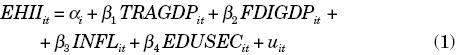
Where EHII is the estimated household income inequality indicator, TRAGDP is the rate of trade to GDP, FDIGDP is the inflow of FDI as a percentage of GDP, INFL shows the annual percentage change of consumer prices, and EDUSEC represents the gross secondary school enrollment as outlined earlier. Subscripts i and t indicate country and year respectively; the error term u_it is assumed to satisfy white noise assumptions; α_i lets the intercept vary for each country and captures country-specific differences; finally, β₁ to β₄ are parameters to be estimated. Previous studies dealing with the effect of market openness on income inequality have applied similar specifications; for instance, IMF (2007) incorporates trade volume and the FDI to GDP ratio as proxies of market openness; in addition, the study includes variables on education, such as population share with at least secondary education and average years of schooling.

II. 1. standard methods

The estimation process starts with the standard OLS method pooling or combining all the observations, and assuming that α_i = α. As column 1 in table 1 illustrates, all the variables are, individually, statistically significant. However, the traditional OLS approach has one major drawback. it assumes that the intercept value of the countries is the same, and there-fore does not control for country-specific factors. So as to confirm whether this is an implausible characteristic of the model, the Breusch and Pagan Lagrange Multiplier test (1980) (LM) is conducted.³ in this case, the result of the test indicates that there are country-specific factors in the model, and therefore the regression with a single constant term is inappropriate.⁴ Hence, we turn to panel estimation methods that may take into account the specific nature of the countries.

The fixed-effects model (FEM) lets the intercept vary for each country by adding dummy variables that take into account country-specific effects. in the Random-effects model (REM), differences across countries are captured through a disturbance term ω_it, which follows ω_it = ε_i + u_it, where ε_i is an unobservable term that represents the individual-specific error component, and u_it is the combined time series and cross-section error component. The REM assumes that ε_i is not correlated with any explanatory variable in the equation.

In order to choose between the FEM and the REM, we apply the Hausman test for specification (1978). The null hypothesis underlying this test is that the regressors and the unobservable individual specific random error are uncorrelated. if the test statistic, based on an asymptotic X² distribution, rejects the null hypothesis, then the random-effects estimators are biased and the fixed-effects model is preferred. The result of the Hausman test from equation (1) suggests that the REM estimates are inconsistent and the FEM would thus be more appropriate.⁵ Since the LM test suggests that there are individual effects, and the Hausman test emphasizes that these effects are correlated with the other variables in the model, it is possible to conclude that, of the alternatives previously considered, the FEM is a better choice. Column 2 in table 1 shows the results from this model.

Before adopting FEM as the final estimation procedure, it is important to conduct an additional test in equation (1). it has already been contended that the error term u_it is assumed to satisfy white noise assumptions, and that it is independently and identically distributed with zero mean, constant variance σ², and serially uncorrelated, which is denoted as u_it ~I.I.D. (0, σ²). By the same token, an AR(1) (autoregressive process of order one) test should be available. in the presence of autocorrelation, both σ² and the standard errors are likely to be underestimated and biased, which leads to misleading conclusions about the statistical significance of the estimated regression coefficients. The test for first-order serial autocorrelation is not satisfied, as it rejects the null: no evidence of AR(1) or ρ = 0.⁶ The P value of the test is also presented in column 2, table 1. To deal with this problem, it is essential to explore the possibility that autocorrelation may arise due to model misspecification; to be precise, because of omitted lagged dependent variables. in this context, equation (1) is extended and transformed into a dynamic panel data model (DPDM) by adding a lagged dependent variable, as follows:

However, the inclusion of a lagged dependent variable introduces a source of persistence over time: correlation between the right hand regressor EHII_it-1 and the error term u_it. furthermore, DPDM is characterized by individual effects η_i caused by heterogeneity among the individuals.⁷ As a con-sequence, it is necessary to adopt different estimation and testing procedures for this model.

II.2. The sys-GMM method

In order to estimate the model, we use a system generalized method of moments (sys-GMM) estimation for DPDMs, initially proposed by Arellano and Bover (1995). firstly, the estimation method eliminates country-effects η_i by expressing equation (2) in first differences, as follows:

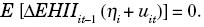
Where X is the set of explanatory variables outlined earlier. On the basis of the following standard moment condition:

That is, lagged levels of EHII_itare uncorrelated with the error term in first differences; the method uses lagged endogenous variables as instruments to control for endogeneity of the lagged dependent variable, reflected in the correlation between this variable and the error term in the transformed equation. The resulting GMM estimator is known as the difference estimator.

Blundell and Bond (1998, pp. 115-116) contended that the GMM estimator obtained after first differencing has been found to have large finite sample bias and poor precision. They attribute the bias and poor precision of this estimator to the problem of weak instruments, as they assert that lagged levels of the series provide weak instruments for the first difference. So as to improve the properties of the standard first-differenced GMM estimator, they justified the use of an extended GMM estimator, on the basis of the following moment condition:

That is, there is no correlation between lagged differences of EHII_it and the country-specific effects. The method therefore uses lagged differences of EHII_it (the endogenous variable) as instruments for equations in levels, in addition to lagged levels of EHII_it as instruments for equations in first differences. The extended sys-GMM encompasses a regression equation in both differences and levels, each one with its specific set of instrumental variables. This type of estimation, called system estimator, not only improves precision and efficiency but also reduces finite sample bias.

The method assumes that the disturbances u_it are not serially correlated. if this were the case, there should be evidence of first-order serial correlation in differenced residuals (u_it- u_it-1), and no evidence of second-order serial correlation in the differenced residuals (doornik, Arellano and Bond, 2002, pp. 5-8). it is an important assumption, because the consistency of the GMM estimators hinges upon the fact that E[Δu_it Δu_it-2] = 0. Accordingly, tests of auto correlation up to order 2 in the first-differenced residuals should be available.

The results of the sys-GMM regression are reported in column 3, table 1. The tests of serial correlation in the first-differenced residuals are in both cases consistent with the maintained assumption of no serial correlation in u_it.The AR(2) test fails to reject the null hypothesis that the first-differenced error term is not second-order serially correlated, whereas by construction, the AR(1) test rejects the null hypothesis that this process does not exhibit first-order serial correlation.⁸

In order to assess the validity of the instruments, a Sargan test of overidentifying restrictions, proposed by Arellano and Bond (1991), is also reported. Under the null hypothesis that the instruments are not correlated with the error process, the Sargan test is asymptotically distributed as a chisquare with as many degrees of freedom as overidentifying restrictions. in this case, the test is unable to reject the validity of the instruments.⁹

The effect of the endogeneity of the lagged dependent variable is that the coefficient on this variable will be biased. in this respect, FEM generates biased estimates when the dimension of T is small, whereas OLS provides biased estimates even when T is large. in our panel, the average T is 14; hence, it is important to know if we can ignore the bias with this size of T or if we can justify the use of instrumental variables, through the application of the GMM approach, in order to control for the correlation between the error term and the lagged dependent variable.

Nickell (1981) derives an expression for the bias of γ and shows that the bias approaches zero as T approaches infinity; the expression is (1/T). in this sense, the magnitude of our average T implies a bias in the coefficient of the lagged dependent variable of 0.071. Judson and Owen (1999) conduct Monte Carlo experiments to address the magnitude of the bias of the OLS and the FEM estimators for various panel sizes. They confirm that using OLS to estimate a model with fixed effects generates a significant bias, even as T gets large. They also show that the FEM bias increases with γ, and in keeping with Nickell (1981) they show that it decreases with T. When N = 100 and γ = 0.8, Judson and Owen illustrate that the magnitude of the FEM bias is 0.232 and 0.104 for T = 10 and T = 20, respectively; in our panel, N = 93 and the average T = 14. They consider a bias above 0.05 as a significant one, and conclude that the GMM technique produces the lowest root mean-squared errors from viable alternatives when ≤ 20.

Hence, the application of a GMM approach is justified because the average T is smaller than 20, the value of γ in FEM is relatively high, 0.63, and according to calculations of Judson and Owen (1999) and the expression derived by Nickell (1981), the bias in the coefficient of the lagged dependent variable in FEM tends to be bigger than 0.05. in particular, we use the sys-GMM estimator because it is designed to improve the properties of the usual first-differenced GMM. it reduces finite sample bias, can be more efficient, and increases precision, as noted earlier.

The dimension of our panel helps to improve the precision of the estimators in relation to other studies on inequality applying the sys-GMM technique (dollar and Kraay, 2004; Felbermayr, 2005), as GMM estimators generally perform better with larger N and T.

 

III. Results

III. 1. original equation

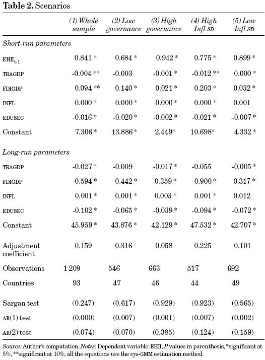
The results are illustrated in table 2. Column 1 shows the results initially obtained by regressing equation (3) with the whole sample. Subsequently, in order to assess the effect of economic liberalization on income distribution under different scenarios of governance and macroeconomic stability, we conducted regressions with four different sub-samples. The first two sub-samples comprise countries with low and high governance; their results are illustrated in columns 2 and 3 respectively. The last two sub-samples contain countries with high and low standard deviation of inflation; their results are shown in columns 4 and 5 respectively. All the equations are regressed using the sys-GMM procedure.

Tables 2 to 6 (3,4,5)incorporate short-run and long-run parameters. following the adaptive expectations hypothesis, first popularized by Cagan (1956) and Friedman (1957), we can interpret the short-run variation on inequality as the increase, sustained during one period only, in the current or observed value of the explanatory variables, times the magnitude of the corresponding short-run parameters. But if the increase in the explanatory variables is sustained over time, then the long-run (or equilibrium) inequality function eventually comprises long-run parameters, which are calculated as follows:

That is to say, when individuals, markets and institutions have time to adjust to the increase in the explanatory variables (sustained across periods), the inequality indicator will increase by the magnitude of the long-run parameters. Section III.3 presents a second strategy to explore long-run effects on inequality by lagging the explanatory variables.

Bearing in mind that a positive sign in the corresponding coefficient indicates a worsening in the distribution of income, the results yield the following conclusions.

Trade. The overall sample indicates that trade reduces income inequality. This finding is in keeping with the expectations supporting trade liberalization, and is also consistent with other studies (Calderón and Chong, 2001; Felbermayr, 2005; IMF, 2007). A 37-unit increase in the rate of trade leads to a long-run decline of 1 point in the income distribution indicator.¹⁰

It should also be emphasized that trade is able to exert a long-term positive impact on income distribution under conditions of macroeconomic balance and high governance. On the other hand, the rate of trade as a percentage of GDP is not significant in countries with macroeconomic distortions and low governance. Thus, the outcome indicates that in the presence of macroeconomic disequilibria and failure of good governance, trade does not exert benefits on income distribution. To some extent, this finding in particular is in accordance with the orthodox assertion that the overall efficiency within a country is an essential factor for the appropriate operation of trade policies.

Investment. The outcome of the overall regression suggests that FDI has an adverse effect on income distribution, and is consistent with previous research (IMF, 2007; Qureshi and Wan, 2008). An upturn of 1.7 points on the rate of investment as a percentage of GDP raises the inequality indicator by 1 point over the long-run. This result undermines the assumptions and expectations outlined in the orthodox postulates.

In addition, table 2 indicates that the effect of FDI is adverse under any scenario. However, if we compare the coefficients across columns 2 to 5, it is possible to observe that this effect is worse in countries with macroeconomic disequilibria and low governance. for example, a 1.7-point upturn in the rate of investment as a percentage of GDP raises the inequality indicator over the long-run by 0.75 and 0.61 points in low and high governance countries respectively, whereas the effects on countries with high inflation and low inflation standard deviation is 1.53 and 0.54 points respectively. Consequently, inefficiency within countries seems to be a factor that accentuates the adverse effect of FDI on income distribution.

So as to test if FDI has an effect on inequality through factors such as geographical location, level of wages or income, and skill supply, three additional regressions are performed; the results are available upon request. firstly, we drop the variable on education from the original equation, and find that the effect of FDI on inequality becomes more adverse in any of the columns; this result suggests that the effect of FDI on inequality can be enhanced by differences in educational levels. Secondly, a variable on the distance from the capital of each country to any of the three major Cities —New York, Tokyo and London— is introduced into the equation; the variable enters positively at significant levels, and it is found that the magnitude of the coefficient on FDI declines. in the third regression, GDP per capita is introduced as a proxy of income level; this variable enters negatively at significant levels, while the magnitude of the coefficient on FDI drops. There-fore, the adverse effect of FDI on income distribution declines when we control for geographical location and level of income, which suggests that difference in these variables also contribute to enhance the effect of FDI.

Inflation. Macroeconomic imbalance is represented by the inflation variable. Results from the overall regression reveal that this variable is a determinant of income inequality. This finding is in accordance with the orthodoxy supporting liberalization and stabilization policies, although the magnitude of the effect is low. An increase in inflation of 930 points, which could be considered an episode of hyperinflation,¹¹ is required to raise inequality by 1 point. Hence, inflation has a negative effect on the distribution of income, but this effect does not seem to be large.

Table 2 reveals that inflation has adverse effects on countries with low governance and macroeconomic distortions. it is worth noting that the repercussions of inflation also affect the distribution of income in countries with high governance. Not surprisingly, this is not significant in column 5; this fact indicates that the inflation rate is a variable that does not affect income distribution in countries that have traditionally kept a stable economy.

In order to test whether inflation is the result of macroeconomic disequilibrium, the following strategy is applied: a proxy of money supply —money and quasi money (M2) annual growth— is added to the original equation. The data source is WDI. The regression is conducted for the over-all sample only, since the number of observations falls to 857. The result shows that the new variable enters positively and significantly in the equation, but inflation is no longer significant. it should be added that the outcome is not owed to the reduction of the sample, but rather on account of the inclusion of the money supply proxy in the equation. As a matter of fact, when we conduct the regression with the same sample but dropping the money supply proxy, the coefficient of inflation is positive and significant. Therefore, the result indicates that inflation has an effect on inequality through the increase in money supply. The same procedure is conducted using a proxy of budget deficit —government expenditure minus tax revenue as a percentage of GDP. The figures are calculated with information from WDI. in this case, the number of observations drops to 697. The outcome indicates that inflation has an effect on inequality through an unbalanced public budget, as the proxy of budget deficit enters positively and significantly to the equation, whereas inflation is no longer significant; moreover, inflation is positive and significant when the proxy of budget deficit is dropped from the equation.¹²

Inflation is used in both ways, as a classification variable and as an explanatory variable, but this approach could create bias in the results. As a classification variable, it captures well the differences on the impact of the variables of interest; on the other hand, the results show low coefficients associated with this variable. Given these results, we substitute inflation with budget deficit as a percentage of GDP as a control for macroeconomic stability, and keep inflation as the classification variable. We find that the coefficient of the budget deficit indicator is only significant in the high governance sub-sample. The same procedure is repeated with the M2 annual growth variable, and we also find that it is significant only in the high governance sub-sample. The lack of significance in these variables is the result of the reduction in the number of observations in each sub-sample. When we examine the magnitude of the coefficients associated with the macroeconomic stability proxies in the whole sample, we find that they are also low. for instance, an upturn of 19 points in the budget deficit as a percentage of GDP is required to raise the inequality indicator by just 1 point over the long-run, while a 732-point upturn in M2 is required to achieve the same long-run effect. Given that the coefficients of these variables are statistically significant in only one sub-sample due to the reduction in the number of observations, and given that they are low and do not capture variations of their effect on inequality across the different scenarios, we keep inflation as the proxy of macroeconomic stability along the paper.

Education. Our results confirm that education reduces income inequality. Similar conclusions have also been obtained in previous studies (de Gregorio and Lee, 2002; IMF, 2007; Teulings and Van Rens, 2008). As for the overall sample, the education coefficient implies that an increase of 10 points in gross secondary school enrollment is required to reduce the inequality indicator by 1 point over the long-run. Moreover, education exerts a positive impact under any scenario. Hence, human capital formation can mitigate the negative effect that may be caused by markets on income distribution, and is in keeping with the postulates of the PWC.¹³

The adjustment coefficient. The outcome of the regressions illustrates that the adjustment coefficient is larger for those countries that exhibit macroeconomic mismanagement or a low level of governance. This fact suggests that these countries are more vulnerable to the effect of the exogenous variables, because their distribution of income adjusts faster to the long-term level, or changes faster compared to those countries with more domestic efficiency.

III.2. Applying changes in trade volume

Some authors contend that trade volume is a variable that reflects countries' geographical characteristics, such as their proximity to major markets, their size, or whether they are landlocked. As a consequence, this variable may tell us little about the effect of trade on growth or income distribution (dollar and Kraay, 2004, p. 26). With the above in mind, "changes in trade volume" is a variable that may eliminate geography or any other unobserved country characteristic. On the other hand, "trade volume" is a variable applied frequently in the empirical literature, including those studies exploring the relationship between economic liberalization and income distribution (Calderón and Chong, 2001). in addition, this variable can be more effective in panel data studies, because they also consider variations over time and not only variations across countries. finally, trade volume improves its explanatory power when it is applied in first difference estimations, such as GMM methods, because in this way unobserved country characteristics are eliminated.

So as to test if our results can vary depending on the applied variable on trade, we regress equation (3), replacing "trade volume" with "changes in trade volume". The outcome of this exercise, including both the overall sample and the four sub-samples, is illustrated in table 3.

It is worth noting that the long-term coefficient of the variable "changes in trade volume" is not significant in the overall sample. This outcome suggests that there is no significant long-term relationship between inequality and changes in trade volume. This finding is consistent with other studies (Dollar and Kraay, 2004). furthermore, "changes in trade volume" is not significant in the sub-samples, except in column 5 of table 3, where the variable enters negatively and at significant levels. Consequently, this result illustrates that countries with macroeconomic stability can improve income distribution due to the expansion of trade. A 36 per cent increase in trade volume leads to a long-term decline of 1 point in income inequality. As for the remaining three variables, they keep the same sign as in the results in table 2, across all the columns, while the magnitude of their coefficients does not differ substantially.

Only in the case of high governance countries (table 3, column 3) there are two variations that deserve highlighting. firstly, the secondary school enrollment variable is not significant. if we consider that high governance countries are associated with high levels of secondary school enrollment and educational attainment, it is likely that an upturn in this variable does not have a considerable impact on income distribution. As a matter of fact, table 2 shows that the coefficient of secondary school enrollment is significant in any scenario, but in the high governance sub-sample it is the smallest compared with the corresponding coefficients in the other sub-samples. in this case, we suggest that higher levels of education can provide more distributional effects. Secondly, the coefficient of the FDI to GDP ratio is not significant either. Thus, when we consider changes in trade volume, FDI does not seem to exert an adverse effect on income distribution in this kind of economies.

In summary, changes in trade volume do not have a significant relationship with income distribution in the overall sample, and, of the four sub-samples, only those countries associated with macroeconomic stability can obtain benefits from the expansion of trade, as table 3 illustrates. in addition, trade volume does not have a significant impact on countries that exhibit domestic inefficiency, but it improves income distribution in the remaining scenarios in table 2. Therefore, there is statistical evidence, emerging from the two variables on trade, which illustrates that countries with domestic efficiency are more likely to improve income distribution on account of an upturn in trade.

The conclusions for all other variables practically do not change, except for the FDI to GDP ratio and secondary school education in high governance countries, as outlined earlier.

III.3. Regional and longer run comparisons

In this section we add regional dummies to the analysis, in order to explore differences in inequality across continents; the benchmark group is European and OECD countries. We also lag the explanatory variables 5 and 10 years, so as to compare their effects in longer run periods. The analysis is conducted for the overall sample. The variable on trade considered here and in the following sections is "trade volume", as it has been shown that its effects do not differ substantially from those using "changes in trade volume".

Column 1 in table 4 indicates that European and OECD countries, as a group, have a more equal income distribution. in contrast, African and Latin American countries appear to have greater income inequality than the benchmark group, by about 4.3 and 5.4 units respectively of the inequality indicator. Asian countries, in average, are slightly more unequal than the benchmark group by 1.9 units of the inequality indicator, but are less unequal than African and Latin American countries in average.

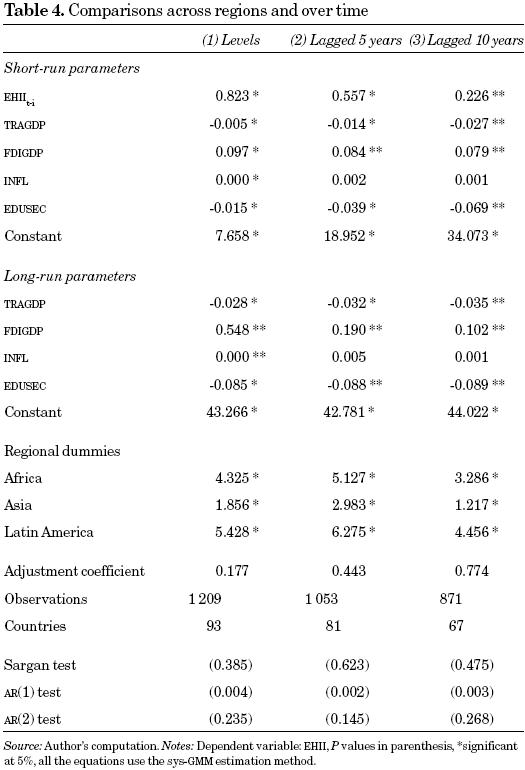
Table A.3 in the appendix shows the average governance indicator and the average standard deviation of inflation for every region. it is possible to observe that regions with low level of governance —Africa and Latin America— are regions with greater inequality, whereas regions with higher level of governance —europe and OECD, and Asia— have a more equal income distribution. furthermore, the Latin American group of countries, which is the most unequal group, has the highest average standard deviation of inflation; in contrast, the group of European and OECD countries has the most stable inflation and the lowest inequality indicator. Hence, good governance and macroeconomic stability can mitigate inequality, and, in fact, are associated with better income distribution.

Columns 2 and 3 in table 4 show the coefficients of the exogenous variables, lagged 5 and 10 years respectively. As before, the equations are estimated with the sys-GMM method, applying instrumental variables, in order to control for endogeneity of the lagged variables. The results indicate that inflation has an adverse effect on income distribution only in the immediate period, represented through the equation in levels in column 1, because in the longer run its coefficient is not statistically significant, as shown in columns 2 and 3. in contrast, the coefficients on trade and education remain significant and negative when these variables are lagged 5 and 10 years; moreover, the magnitude of the coefficients is larger as the lagged period increases. Hence, trade and education can have more redistributional effects in the longer run. As for the coefficient on FDI, it remains significant and positive but the magnitude decreases over time, which suggests that the adverse effect of FDI on inequality tends to decrease in the longer run.

III.4. The effects of exports by sector

Trade openness plays a preponderant role, as it is assumed to give an unambiguous boost to the exportable sector and therefore to export-led growth. in this context, export growth may raise employment directly in the exportable sector and indirectly by permitting faster GDP growth. This process is expected to have positive implications for income distribution and longer-term growth.

We have already contended that according the Stolper-Samuelson and on the basis of the principle of comparative advantage, we may expect that primary exports, based on natural resources and unskilled labor, provide larger benefits to income distribution than manufactured exports in those countries which exhibit low governance and high inflation standard deviation, since these countries are associated with lower levels of development.¹⁴

In order to test the effect of manufactured exports and primary exports on income distribution, we conduct a regression including two variables representing the percentage of manufactured exports and primary exports to merchandise exports. Table 5 illustrates that the proxy of manufactured exports is negative and statistically significant in the overall sample and in the four sub-samples. An upturn of 8.9 points in the rate of manufactured exports to merchandise exports is linked with a long-run decline of 1 point in income inequality in the overall sample. On the other hand, the proxy of primary exports is not significant in any case, not even in the low governance and high inflation variance sub-samples.¹⁵

III.5 The role of employment and government size

It has already been noticed that employment, especially in the primary sector, is deemed to be one of the main factors that can drive a better distribution of income. So as to test this assumption, we extend the original equation by adding a proxy for the level of employment. We include the unemployment rate variable. Results are shown in table 6, column 2. in addition, so as to test the role of employment by sector, we include as variables the ratios of employment by industry and agriculture to total employment. Results are provided in table 6, columns 3 and 4 respectively. finally, we undertake an additional exercise to explore the role of the state and its empowerment in the distribution of income. for this purpose, we use the "government expenditure to GDF " variable. Results are provided in table 6, column 5. in all the equations, the exercise is conducted only for the overall sample because of constraints on data availability. That is, after including the "unemployment", "employment by sector" and "government expenditure" variables, the number of observations drops.

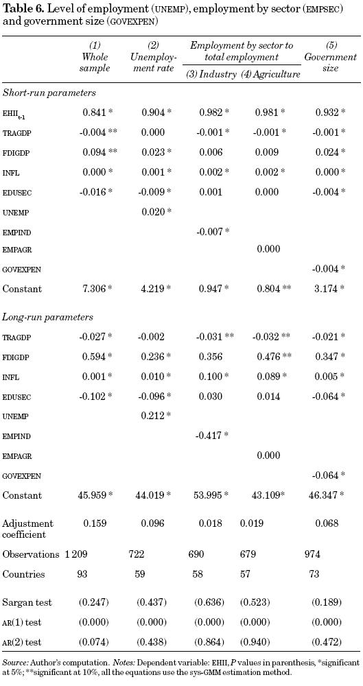
Firstly, we observe that unemployment enters positively and significantly in the equation, indicating that higher levels of employment are associated with less inequality. A 4.75-point reduction of unemployment drops the inequality indicator by 1 point over the long-run. What is striking is that trade volume does not remain significant. However, this result is not owed to the inclusion of unemployment in the equation, but rather on account of the reduction of observations in the sample. As a matter of fact, when we conduct the regression with the same sample comprising 781 observations and dropping the unemployment variable, trade volume is not significant either.

When we explore the effect of employment by sector on income distribution, it is interesting to note that the ratio of "employment in agriculture" to "total employment" is not significant. On the other hand, what is striking is that the ratio of "employment in industry" to "total employment" is significant and negative. An increase of 2.4 points in this ratio is required to reduce inequality by one point over the long-term. it should also be added that the "FDI to GDP" and "secondary school enrollment" variables are no longer significant in this equation. However, as in the case of the "unemployment" variable, this outcome is not due to the inclusion of an additional variable in the equation, in this case "employment in industry". This outcome is rather caused by the reduction of the sample. On the contrary, when the regression is conducted with the same sample (690 observations) but dropping the "employment in industry" variable, both "FDI to GDP" and "secondary school enrollment" are not significant either.¹⁶

In this sense, results in tables 5 and 6 are supportive and complement each other. in table 5 we show statistical evidence suggesting that the growth of manufactured exports decreases inequality, while in table 6 we illustrate that employment in industry is associated with improvements in income distribution. furthermore, both variables can have longer run effects on inequality. in contrast, from the two previous tables there is not statistical evidence suggesting that primary exports and employment in agriculture can reduce inequality, even in those countries associated with lower levels of development and abundant unskilled labor, such as countries with low governance and high inflation standard deviation.

As for the proxy for government size, it enters negatively and significantly, while the other variables remain significant. An upturn of 15 points on government expenditure drops the inequality indicator by 1 point over the long-run. it should be added that the estimated results may be biased by the potential endogeneity of government expenditure. Moreover, it is not obvious that a strong state with high government expenditure reduces inequality; it may well be that high level of government transfers, correlated with a high government expenditure ratio, can reduce inequality. in order to address this issue, government size is instrumented. We use subsidies and other transfers (percentage of GDP), where available, as an instrument of government expenditure; the variable is calculated with information from WDI. The regression shows a similar pattern of results to those presented in Table 6. The exception is that the impact of the instrumental variable on inequality is rather higher than that of government expenditure. On the other hand, if we introduce both variables in the equation simultaneously to test which one is more robust, we find that no one is significant. This outcome is the result of a reduction in the number of observations, given that the instrument is only available for around 60 per cent of the sample of column 5 in table 6. Hence, the re-empowerment of the state, and in particular a high level of subsidies and transfers, are factors that can improve income distribution.¹⁷

 

IV. Concluding remarks

From the statistical evidence presented above, we find a negative relationship between trade and inequality, especially in those countries with evidence of domestic efficiency. When the analysis of trade is extended by sectors, the results illustrate that an exportled growth strategy based on the primary sector does not improve income distribution, whereas manufactured exports can reduce inequality; the results apply even in those countries associated with lower levels of income. We also find that the impact of FDI on income distribution is adverse, because it does not provide distributional effects. it is worth noting that differences in education and level of income across countries and over time, and different geographical location across countries, enhance the adverse effect of FDI on income distribution. in order to have a better perspective of the effect of the economic prescription embedded in the Washington Consensus, other variables, such as inflation and employment, are incorporated in the study. inflation increases inequality, but only through episodes of hyperinflation. This variable can be considered a proxy of macroeconomic disequilibrium, as it is shown in the paper that inflation has an effect on inequality through the increase of money supply and through an unbalanced public budget. Higher levels of employment are associated with less inequality; more-over, the sectoral analysis of this variable shows that employment in industry can have better consequences for income distribution than employment in agriculture.

Consequently, the empirical evidence obtained from this study is in keeping with the assumptions and expectations supporting market liberalism to the extent that trade, employment and low inflation can benefit income distribution. in contrast, the results undermine these assumptions and expectations in the sense that FDI worsens inequality. in addition, an exportled growth strategy and the expansion of employment supported on the primary sector do not provide the basis for redistribution.

On the other hand, countries with macroeconomic stability and high governance can mitigate the adverse effect of FDI on income distribution, while there is evidence that they can obtain benefits from trade. in contrast, countries that exhibit domestic inefficiency do not benefit from trade, and the effect of FDI on their distribution of income is worse. it is also worth noting that inflation does not worsen inequality in those countries associated with a stable economy. We also find that a strong state, associated with high levels of government expenditure and in particular with high levels of subsidies and transfers, can achieve distributional effects. finally, the study confirms that education can socialize the operation of market forces, since it reduces inequality. in short, domestic efficiency, the empowerment of the state, and emphasis on second generation policies (represented in this study by a proxy of human capital formation) can mitigate the adverse effect of economic liberalization on income distribution, and to some extent can reduce inequality. Consequently, the study shows that the PWC represents an improvement to socialize the functioning of markets. Nevertheless, the results suggest that the role of the state is not enough because, even under conditions of macroeconomic stability and high governance, FDI does not benefit income distribution. for these reasons, we argue that further supranational mechanisms, beyond the scope of the state, are required to obtain distributional effects from the flow of FDI.

Through the regional analysis it is confirmed that stable inflation and good governance tend to be positively correlated with better income distribution. finally, the longer run comparisons conducted in the study, by lagging the explanatory variables, reveal that trade in general (more specifically manufactured exports) and employment in industry can have more redistributional effects over time, while the adverse effect of both FDI and inflation decreases. Moreover, education and government expenditure keep their benefit in the longer run. Hence, the operation of markets can have better consequences for redistribution in the longer run, and there is evidence that emphasis on manufacturing and industrial activities, and the action of an efficient state, enhance the benefits.

 

References

Arellano, M. and O. Bover (1995), "Another Look at the instrumental Variable estimation of error-component Models", Journal of Econometrics, 68, pp. 29-51.         [ Links ]

Arellano, M. and S. Bond (1991), "Some Tests of Specification for Panel data: Monte Carlo evidence and an Application to employment equations", The Review of Economic studies, 58 (2), pp. 277-297.         [ Links ]

Baltagi, B. H. (2001), Econometric Analysis of Panel Data, 2^nd ed., Sussex, John Wiley & Sons.         [ Links ]

Blundell, R. and S. Bond (1998), "Initial Conditions and Moment Restrictions in dynamic Panel data Models", Journal of Econometrics, 87, pp. 115-143.         [ Links ]

Breusch, T. and A. Pagan (1980), "The lm Test and its Applications to Model Specification in econometrics", The Review of Economic studies, 47, pp. 239-254.         [ Links ]

Cagan, P. (1956), "The Monetary dynamic of Hyperinflation", in M. Friedman (ed.), Studies in the Quantity Theory of money, Chicago, University of Chicago Press.         [ Links ]

Calderón, C. and A. Chong (2001), "External Sector and income inequality in interdependent economies Using a dynamic Panel data Approach", Economics Letters, 71, pp. 225-231.         [ Links ]

Camdessus, M. (1998), "Income distribution and Sustainable Growth: The Perspective from the IMF at fifty", in V. Tanzi and K.-Y. Chu (eds.), Income Distribution and High-Quality growth, Massachusetts, MIT Press, pp. XI-4.         [ Links ]

De Gregorio, J. and J.-W. Lee (2002), "Education and income inequality: New evidence from Cross-country data", Review of Income and Wealth, 48 (3), pp. 395-416.         [ Links ]

Deininger, K. and L. Squire (1996), "A New data Set Measuring income inequality", The World Bank Economic Review, 10 (3), pp. 565-591.         [ Links ]

–––––––––– (1998), "New Ways of Looking at Old issues: inequality and Growth", Journal of Development Economics, 57, pp. 259-287.         [ Links ]

Distance Calculator (2009), http://www.mapcrow.info/.         [ Links ]

Dollar, D. and A. Kraay (2004), "Trade, Growth, and Poverty", The Economic Journal, 114, pp. 22-49.         [ Links ]

Doornik, J. A., M. Arellano and S. Bond (2002), Panel Data Estimation using DPD for ox, Centro de Estudios Financieros y Monetarios.         [ Links ]

Edwards, M. (1999), Future Positive: International cooperation in the 21^st century, London, Earthscan.         [ Links ]

Felbermayr, G. J. (2005), "Dynamic Panel data evidence on the Trade-income Relation", Review of World Economics, 141 (4), pp. 561-760.         [ Links ]

Friedman, M. (1957), A Theory of the consumption Function, National Bureau of economic Research, Princeton, Princeton University Press.         [ Links ]

Galbraith, J. K. and H. Kum (2002), Inequality and Economic growth: Data comparison and Econometric Tests, University of Texas inequality Project, UTIP working paper 21.         [ Links ]

–––––––––– (2003), Estimating the Inequality of Household Incomes: Fillinggaps and correcting Errors in Deininger & squire, University of Texas inequality Project, UTIP working paper 22.         [ Links ]

Gilpin, R. (1987), The Political Economy of International Relations, Princeton, Princeton University Press.         [ Links ]

Greene, W. H. (2008), Econometric Analysis, 6^th ed., New Jersey, Prentice Hall.         [ Links ]

Hausman, J. A. (1978), "Specification Test in econometrics", Econometrica, 46, pp. 1251-1271.         [ Links ]

Havrylyshyn, O., M. Miller and W. Perraudin (1994), "Deficits, inflation and the Political economy of Ukraine", Economic Policy, 19, pp. 353-401.         [ Links ]

Heerink, N. (1994), Population growth, Income Distribution, and Economic Development: Theory, methodology, and Empirical Results, New York and Berlin, Springer.         [ Links ]

Higgott, R. (2000), "Contested Globalization: The Changing Context and Normative Challenges", Review of International studies, 26, pp. 131-153.         [ Links ]

Higgot, R. and N. Phillips (2000), "Challenging Triumphalism and Convergence: The Limits of Global Liberalization in Asia and Latin America", Review of International studies, 26, pp. 359-379.         [ Links ]

International Monetary Fund (1997), World Economic outlook: globalization and the opportunities for Developing countries, May, chapter 4.         [ Links ]

–––––––––– (2007), World Economic outlook: Globalization and inequality, October, chapter 4.         [ Links ]

Jha, S. (1996), "The Kuznets Curve: A Reassessment", World Development, 24 (4), pp. 773-780.         [ Links ]

Judson, R. A. and A. L. Owen (1999), "Estimating dynamic Panel data Models: A Guide for Macroeconomist", Economics letters, 65, pp. 9-15.         [ Links ]

Kaufmann, D., A. Kraay and P. Zoido-Lobaton (1999), Governance Matters, World Bank Policy Research Working Paper 2196.         [ Links ]

Luxembourg income Study (LIS) (2007), The LIS Database.         [ Links ]

Ma, Alyson C. (2006), "Geographical Location of foreign direct investment and Wage inequality in China", World Economy, 29 (8), pp. 1031-1055.         [ Links ]

Milanovic, B. (1995), Poverty, Inequality and social Policy in Transition Economies, World Bank, Transition economics division, Research Papers 9.         [ Links ]

Nickell, Stephen J. (1981), "Biases in dynamic Models with fixed effects", Econometrica, 49, pp. 1417-1426.         [ Links ]

Ortiz, G. (2003), "Latin America and the Washington Consensus: Overcoming Reform fatigue", Finance and Development, 40 (3), pp. 14-17.         [ Links ]

Qureshi, M. S. and G. Wan (2008), "Distributional Consequences of Globalization: empirical evidence from Panel data", Journal of Development studies, 44 (10), pp. 1424-1449.         [ Links ]

Redding, Stephen and Anthony J. Venables (2004), "Economic Geography and international inequality", Journal of International Economics, 62 (1), pp. 53-82.         [ Links ]

Teulings, C. and T. Van Rens (2008), "Education, Growth and income inequality', Review of Economics and statistics, 90 (1), pp. 89-104        [ Links ]

UNESCO Institute for Statistics (2007), Statistical Tables.         [ Links ]

United Nations Conference on Trade and Development (2007), Foreign Direct Investment Database.         [ Links ]

United Nations University and World Institute for Development Economics Research (2007), World Income Inequality Data Base.         [ Links ]

University of Texas inequality Project (2002), UTIP–UNIDO Database.         [ Links ]

Williamson, J. (1990), "What Washington Means by Policy Reform", in J. Williamson (ed.), Latin American Adjustment: How much Has Happened? Washington, D. C., Institute for International Economics, pp. 7-20.         [ Links ]

World Bank (2007), Worldwide governance Indicator.         [ Links ]

World Bank (2007), World Development Indicators 2007, CD-ROM, Washington, D. C., World Bank.         [ Links ]

Wu, Xiaodong (2001), Impact of FDI on Relative Return to skill, University of North Carolina at Chapel Hill Working Paper.         [ Links ]

 

Notas

¹ John Williamson (1990) is given credit for first labelling as Washington Consensus the package of policies that multilateral institutions endorsed in trade and loan negotiations during the 1980s. This package of policies insisted on unregulated markets and a reduced role of the governments in economic activity.

² Cluster analysis is a set of algorithms that put objects or data into groups according to similarity rules. in particular, the K-means algorithm assigns each point to the cluster whose center is nearest. The center is the average of all the points in the cluster.

³ The LM test, based on the OLS residuals and under the null hypothesis (α_i = α, that is, the classical regression model with a single constant term is appropriate), is distributed as a X² with one degree of freedom (Greene, 2008).

⁴ We obtain a Lagrange Multiplier test statistic of 4 466, which far exceeds the 5 per cent critical value of X² with one degree of freedom, 3.84. Since the null hypothesis is rejected, it is concluded that there are individual effects.

⁵ The value of the Hausman test statistic is 130.65 with a negligible P value; hence, the test rejects the null hypothesis. in this case, the key assumption of the REM "the unobservable individual-specific error ε_i is not correlated with any explanatory variable" is violated; thus, the FEM is preferred.

⁶ The AR test statistic of order one is equal to 29.99, and the P value is negligible. Hence, the AR(1) test suggests evidence of first-order autocorrelation.

⁷ For an elaboration in this point see Baltagi (2001, pp. 129-130).

⁸ The P value in the test statistic for second-order serial correlation, based on residuals from the first-difference equation, is equal to 0.074. in this case, we cannot reject the null hypothesis if we establish a 95 per cent confidence interval. even in these circumstances, the sys-GMM model represents a substantial improvement in terms of ar compared with ordinary methods. The P value in the test statistic for first-order serial correlation is negligible; in this case, the null hypothesis is rejected at any conventional level of significance.

⁹ The Sargan test statistic is equal to 55.38 with a P value equal to 0.247. Thus, the test is unable to reject the hypothesis that the instruments are not correlated with the error process.

¹⁰ This figure is obtained by dividing the short run parameter of the corresponding variable by 1 minus the coefficient of the lagged dependent variable, times the magnitude of the increase in the corresponding exogenous variable, as follows: ((0.004/(1-0.841))*37).

¹¹ Hyperinflation is a very high increase in the aggregate price level when inflation is out of control. Although the threshold to define hyperinflation is arbitrary, the threshold customarily used is an increase of prices averaging 50 per cent a month (Havrylyshyn, Miller and Perraudin, 1994). in this sense, a good that costs £1 in January would cost £130 in January of the next year.

¹² Inflation can be affected by large swings in energy prices in the longer run; however, we do not test this possibility due to constraints in data availability. Nevertheless, our results indicate that inflation has an effect on inequality through macroeconomic mismanagement on a year to year basis, but inequality seems to be affected only in episodes of hyperinflation.

¹³ As complementary information, we found that a lower rate of population growth leads toward less inequality, as the corresponding coefficient enters positively and significantly in the overall sample and the four sub-samples. in this context, Heerink (1994) shows that income inequality and population growth reinforce each other, because lower levels of fertility result in a more equal income distribution; he also underlines the negative relationship between improvements in nutrition, health and education on the one hand and the fertility levels on the other. Not surprisingly, our database also reveals a negative relationship between education and the rate of population growth. These findings suggest that education can contribute directly to improve income distribution, but also contributes indirectly to this effect by reducing the rate of population growth.

¹⁴ Kaufmann, Kraay and Zoido-Lobaton (1999) provide evidence of a strong positive relationship between governance and better development outcomes. in this sense, countries with a low level of governance are associated with a low level of development, and therefore they can have substantial reliance on natural resources and unskilled labor.

¹⁵ As in table 4, the explanatory variables are lagged 5 and 10 years to analyze their longer run effect on inequality. The exercise is conducted only for the overall sample due to a reduction in the number of observations. We found that the proxy of primary exports is not significant in any of the two lagged periods. in contrast, the proxy of manufactured exports is significant and positive in both lagged periods. Consequently, manufactured exports can have longer run benefits on income distribution.

¹⁶ in order to test the longer run effect of the explanatory variables, we lagged them only 5 years because the size of the sample drops substantially when the explanatory variables are lagged 10 years. Only the coefficients in the ratio of employment in industry and government expenditure are significant and keep their negative sign.

¹⁷ Throughout the paper, several attempts have been made to address the issue of endogeneity. in this sense, variables such as FDI, inflation and the government size were replaced by their instruments, or their instruments were added to the equations, in order to explore those channels through which the exogenous variables influence income distribution. Nevertheless, the problem of endogeneity might persist because other relevant instrument variables (such as corporate tax rate as an instrument of FDI, public expenditure on health and education as an instrument of government size, and commodity prices and energy prices as instruments of inflation) have not been incorporated into the analysis due to constraints in data availability.