Seasonal and annual regional drought prediction by using data-mining approach

 

K. Yurekli
Department of Biosystem Engineering, Faculty of Agriculture, University of Gaziosmanpasa,
60240 Tasliciftlik, Tokat, Turkey

M. Taghi Sattari
Department of Water Engineering, Faculty of Agriculture, University of Tabriz, Tabriz 5166614766, Iran

A. S. Anli
Department of Farm Structure and Irrigation, Agriculture Faculty, University of Ankara, Ankara-Turkey

M. A. Hinis
Department of Civil Engineering, Faculty of Engineering, University of Aksaray, Aksaray-Turkey
Corresponding author; e-mail: mhinis@gmail.com

 

Received March 3, 2010; accepted July 29, 2011

 

RESUMEN

Este estudio examina el análisis de la sequía estacional regional con base en el método del índice estandarizado de precipitación (SPI, por sus siglas en inglés) y en la técnica del árbol de decisiones que es una aproximación de minería de datos. Se formaron series de precipitación acumulada para cinco periodos de referencia (cuatro series estacionales y una anual) utilizando la precipitación mensual de 17 estaciones de la cuenca de Cekerek en Turquía, que tiene un área de 1 165 440 ha. Se realizó un análisis regional agrupando las estaciones inicialmente como grupos homogéneos de acuerdo con el criterio de discordancia considerando las tasas de momento-l. No hubo estaciones discordantes de acuerdo con las medidas de discordancia de las características de los sitios, excepto para las del primer período de referencia. Las medidas de heterogeneidad muestran que los grupos seleccionados fueron homogéneos. Con base en el criterio de bondad de ajuste |ZDIST| las distribuciones regionales candidato con |ZDIST| mínimo para los periodos de referencia k fueron la Pareto generalizada (GPA), la de valores extremos generalizados (GEV), la logística generalizada (GLO) la Pearson tipo III (PE·), la GEV y la log normal de 3 parámetros (LN3), respectivamente. Las categorías de sequía para cada región se predijeron aplicando el árbol de decisiones obtenido de la fase de entrenamiento para los periodos k de referencia. Los resultados revelan que no hubo diferencia significativa entre las categorías de sequía calculadas con el algoritmo convencional de SPI y las de la aproximación por el árbol de decisiones. Más aún, la exactitud de la predicción para los periodos de referencia k fue mayor que 94 %, excepto para los períodos de referencia k3 (81.2 %) y k5 (86.4 %).

 

ABSTRACT

This study examines the seasonal regional drought analysis based on the standardized precipitation index (SPI) method and the decision tree technique which is a data-mining approach. The cumulative rainfall series for five reference periods (four seasonal and one annual series) were constituted by using monthly rainfalls from 17 stations in Cekerek Watershed, Turkey, which has an area of 1165 440 ha. Regional analysis was performed by forming the stations initially as homogeneous group(s) according to the discordancy criteria considering by l-moment ratios. There was no discordant station according to discordancy measure of site characteristics except for the first reference period. The heterogeneity measures showed that the selected groups were homogeneous. Based on the goodness of fit criteria |Z^DIST| the candidate regional distributions having the minimum Z^DIST for k-reference periods were the Generalized Pareto (GPA), Generalized Extreme Values (GEV), Generalized Logistic (GLO), Pearson Type III (PE3), GEV and 3-parameter Log Normal (LN3), respectively. The drought categories for each region were predicted by applying the decision tree rules obtained from the training phase of the k-reference periods. The results revealed that there was no significant difference between drought categories calculated from the conventional SPI algorithm and decision tree approaches. Moreover, the accuracy of prediction for k-reference periods was greater than 94%, except for k3 (81.2) and k5 (86.4%) reference periods.

Keywords: L-moments, regionalization, standard precipitation index, decision tree.

 

1. Introduction

Drought is one of the most serious problems for human societies and ecosystems arising from climate fluctuations and variations. Although its impact does not come through sudden events, such as floods and storms, drought is one of the most damaging types of natural disasters influencing for longer periods. Initiation of drought is less noticeable and there are no rapid physical disruptions at the beginning. However, droughts may become disastrous in time and spread into wide areas by affecting many more social, economical and environmental aspects than other types of disasters do. Drought can last for long time and sustain the impact for longer durations. Human interferences often increase the impact of drought because of a high use of water that cannot be supported when the natural supply is limited. Although it is not easy to define droughts precisely, they can be simply considered as periods of insufficient precipitation and water supply relative to average conditions, however, operational definitions may often help to define the onset, severity and end of droughts. Le Houerou (1996) stated that droughts were experienced in almost all types of agricultural land in the world, but arid lands are most susceptible.

Drought is classified as agricultural, hydrological or meteorological. Agnew and Warren (1996) described agricultural drought as a spatial phenomenon that causes significant reductions in agricultural productivity, mainly due to an inadequate supply of soil moisture. Hydrological drought refers to deficiencies in surface and subsurface water supplies (Palmer, 1965). Meteorological drought is usually measured by how far the precipitation from normal has been over a certain period of time (Agnew, 1990).

Numerous indices were designed to quantify agricultural, hydrological and meteorological droughts. Drought indices derived from hydroclimatical data are supposed to provide a concise information about the drought condition of a region. These indices are aften used for making decisions on water resources management and water allocations for minimizing the impact of drought. Researchers have focused on standardized precipitation index (SPI) recently to examine the problems such as drought, flood and crop yields. SPI quantifies the precipitation deficit and may be applied in areas with different climates for various time scales (Edwards and McKee, 1997). SPI is based on the monthly precipitation data summed at different time scales and fitted to a statistical distribution.

Loukas and Vasiliades (2004) examined the temporal and spatial characteristics of meteorological drought to provide a framework for sustainable water resources management in the region of Thessaly, Greece by using the SPI as an indicator of both the drought severity and the characteristics of droughts. Yamoah (2000) investigated the effects of the SPI and fertilizer nitrogen (N) rate on yield and risk of maize-based cropping systems in northeast Nebraska. They expressed that the SPI would be used as an indicator to choice of crops, N levels, and management decisions to conserve water in rainfed cropping systems. Selier (2002) used the SPI as a tool for monitoring flood risk affecting the southern Cordoba province in Argentina. Giddings (2005) implied that the SPI were used with notable success in various applications as an indicator of drought severity or excessive wetness. Alatise and Ikumawoyi (2007) applied four techniques namely, the Stochastic Component Time Series (SCTS), the Rainfall Anomaly Index (RAI), the Cumulative Rainfall Information (CRI) and the Drought Severity Index (DSI) to a 73-year rainfall data for the evaluation of drought in Lokoja, Nigeria. The RAI was selected as the most appropriate technique because of its ability to supply more information on drought occurrences in the study area more than the other three techniques. Oladipo (1985) examined the performances of three drought indices, namely the RAI, Bhalme and Mooley drought index (BMDI) and the Palmer drought index (PDI) and stated that the three indices appeared to be effective in detecting drought periods. Wu et al. (2004) developed an agricultural drought risk-assessment model for corn and soybeans by using the standardized precipitation index and crop-specific drought index. The 26-time scales of the SPI were included for this reason, and the SPI values at four time scales (4, 10, 32 and 52 weeks) were selected for model development. Labedzki (2007) estimated meteorological drought frequency in the region of Bydgoszcz in the central part of Poland by taking into consideration the SPI values at 3-, 6-, 12-, 24- and 48-month timescales.

In this study, regional drought analysis based on the SPI method and data mining approach were carried out. Large historical datasets are required to identify the complex inter-relationship between different climatic parameters and to distinguish patterns that may be used to predict drought. In this sense, an automated and efficient way is desired to extract reasonable information from such large data archives. This problem can be overcome by using data mining approach, which is a relatively new method developed for extracting relevance information from large datasets. Tadesse (2004) reported that data mining approach was used for commercial applications, medical research, and telecommunications, but it was not for drought analysis. Therefore, they analyzed the usability of the technique to find associations between drought and several oceanic and climatic indices, and suggested that data mining technique could be used to monitor drought. Sharma (2006) used the SPI and Vegetation Condition Index (VCI) as input parameters for generating the rules related to data mining, and concluded that data mining technique by using association rule and independent component analysis was successfully applied, and it was possible to extract information about the temporal and spatial pattern of drought. Belda and Penades (2007) examined data mining by using OLAP-mining technique to determine the association rules between synoptic patterns and climatic index.

Main objective of the present study is to perform seasonal and annual regional drought analysis based on SPI by means of decision tree technique which is a data-mining approach. The study was arranged in four consecutive stages as follows. The first step was to constitute the cumulative rainfall series for the k-reference periods by using monthly rainfalls from 17 stations in Cekerek Watershed. The second stage was to form sub-homogeneous regions for the regional frequency analysis and to choose the best fit regional distribution for the cumulative rainfall series obtained from the stations in the sub-homogeneous regions. The third stage was to transform the cumulative rainfall series in the sub-homogeneous region to normal (Gaussian) symmetrical distribution by using the candidate regional distribution to find the z-score (SPI) relationship. The SPI classification suggested by McKee et al. (1993) is given in Table I. In the last stage, the decision tree technique was applied to the cumulative rainfall series to delineate drought categories based on the SPI values.

 

2. Materials and methods

2.1 Cekerek watershed

The Çekerek Stream watershed lies in between 39º 30' and 40º 45' N and 35º 15' and 36º 15' E. This area covers approximately 1165 440 ha, which is about 1.5% of Turkey's total area. The study area is located on the north Anatolia fault line that is one of the most effective faults in the world. Therefore, tectonic movement affects the characteristics of the watershed. The Çekerek Stream is formed by the confluence of small streams that originate from the Kizik, Dinar, Çali and Kavak hills, near the Çamlibel district. The Çekerek Stream is approximately 276 km in length. The stream drains into the Yesilirmak River near Kayabasi (Anonymous, 1970). In this study, four seasonal (SRS) and one annual rainfall (ARS) series were formed by using monthly total precipitation series obtained from 17 selected rain gauge stations in the Cekerek watershed, Turkey. The selected 17 stations, managed by the Turkish State Meteorological Service and General Directorate of State Hydraulic Works, were scattered over the Cekerek watershed to represent fully the precipitation regimes affecting the area. The approximate locations of the rain gauge stations are shown in Figure 1. There is a lack of data in monthly total rainfalls of some years for some of the rain gauge stations in the studied region. The year of interest was discarded for the k-reference period with lack of the data. The data records of 17 stations were given in Table II.

 

2.2 Analysis of data

It is assumed that a time series of monthly rainfall depths, P_i,j, is available where i denotes the year and j denotes the month. The seasonal rainfall depth series for the k-th reference period is obtained as:

and annual rainfall depth series is obtained as

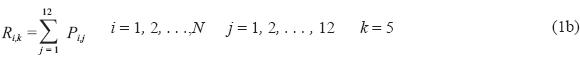
where R_i,k is the cumulative rainfall depth for the k-th reference period of i-th year, k = 1 for January-March, k = 2 for April-June, k = 3 for July-September, k = 4 for October-December and k = 5 for January-December (annual) time periods.

 

2.3 Standardized precipitation index (SPI) algorithm

The SPI developed by McKee (1993) is a way of measuring drought characteristics based only on precipitation data. The SPI is used to monitor conditions on a variety of time scales. Technically, the SPI is the number of standard deviations that the observed value would deviate from the longterm mean, for a normally distributed random variable. The SPI have some advantages for the following reasons. Precipitation is the only variable in the SPI calculation. Therefore, this index can be applied to any regions where the availability of climatic variables limits the use of other widely used indices such as Palmer Drought Index (PDI). To have a wide spectrum of time scales make SPI more flexible for both short-term and long-term drought monitoring than any other indices (Edwards and McKee, 1997; Redmond, 2000). Alley (1984) and Guttman (1998) compared SPI and PDSI, and spatial inconsistency was found in PDSI, thefore SPI was recommended for drought studies. SPI is comparable both in time and space and is not affected by geographical or topographical differences (Lana, 2001). The SPI algorithm is conceptually equivalent to z-scores commonly used in statistics:

where, SPI represents the standardized precipitation index, p_i is the rainfall for a given period, n is the total length of record and σ_p is the standard deviation.

McKee (1993) used the drought classification system shown in Table I to define intensities resulting from the SPI. A drought event occurs any time when the SPI is continuously negative and reaches an intensity where the SPI is -1.0 or less. The event ends when the SPI becomes positive.

It is known that rainfall data is typically positively skewed. Therefore, the precipitation data should be transformed to a more normal or Gaussian symmetrical distribution to use the z-score relationship. McKee (1993, 1995) and Komuscu (1999) implied that the long-term rainfall data sets must be first normalized to determine the SPI of the data sets. The application of many researchers related to the transformation of monthly rainfall is the gamma distribution. Thom (1966) stated that monthly rainfall generally fit to the gamma distribution. Guttman (1999) examined impact of six distributions on SPI and recommended that Pearson Type III distribution is the best way to normalize long-term data when calculating SPI. Edwards and McKee (1997) suggested gamma distribution with two parameters to transform the precipitation data. Kumar (2009) investigated the use of SPI for drought intensity assessments and found that SPI values calculated by gamma distribution underestimate dryness and wetness caused by very low and very high rainfall. Therefore they stated that there is a need to use other statistical distributions for SPI computation for improving the sensitivity.

Before executing the transformation, it is an important task to find the best distribution representing the precipitation data since it has an impact on the SPI. Therefore, it was decided to use the l-moment approach introduced by Hosking (1990) to choose the best fit regional distribution in the study.

 

2.3.1 l-Moment approach

The l-moments are first defined by Hosking (1990) as an alternative approach of describing the shape of probability distributions. They are analogous to conventional moments with measures of location, scale and shape, and able to be computed from linear combinations of order statistics. The l-moments have some theoretical advantages over conventional moments. These advantages are that they are mostly robust and less sensitive to outliers, so that l-moments are calculated as linear combination of the ordered data sequence unless squaring or cubing the data. Moreover, the parameter estimations are more reliable than the conventional method of moment estimates, particularly from small samples, and are usually computationally more tractable than maximum likelihood estimates. On the other hand, estimators of l-moments are virtually unbiased (Hosking and Wallis, 1997). Basically, l-moments are linear functions of probability weighted moments (PWMs). The PWMs are defined by Greenwood (1979) as;

Where ß_rj is the r^th order PWM at site j and F_j(x_j) is the cumulative distribution function (cdf) of x_j at site j. For any given site, the four first l–moments based on the PWMs are defined;

The l-moment ratios are l-coefficient of variation (l-Cv; τ₂ = λ₂/λ₁), l-skewness (l-Cs; τ₃ = λ₃/λ₂) and l-kurtosis (l-Ck; τ₄ = λ₄/λ₂), respectively.

 

2.3.2 Regionalization

Researchers have focused on spatial variability of hydrological response of a given region to delimitate homogeneous hydrological regions called as hydrological regionalization. The definition of a homogeneous hydrological region is that the sites in that region show spatially a high degree of similarity from the hydrological response point of view. Thus, the limited information available at a site is able to be augmented and enhanced with information available at other sites in the homogeneous region. Therefore, many approaches related to regionalization were developed, in the recently, the most popular of them is regionalization based on l-moments. The regionalization procedure used in this study is outlined below.

 

2.3.3 Discordancy measure

Main objective of this analysis is to identify any site in the selected region in three-dimensional space. The discordancy measure Di (Hosking and Wallis, 1997) compares the L-moment ratios of a site with those of the pooling group as a whole. If a given site is not in the cloud of (τ₃, τ₄) points on the l-moment diagram, that is, is far from the center of the cluster, the site is removed to other region. The sites in the homogeneous region (pooling group) form a cluster. Discordancy measure (D_i) of a site can be calculated by

Where u is the vector of l-moments, and N is the number of stations. For N315, Di should be less than or equal to 3.

 

2.3.4 Heterogeneity analysis

Hosking and Wallis (1993) recommended heterogeneity (H) test to assess whether the regions proposed as homogeneous according to discordancy measure of site characteristics are reasonably treated as a homogeneous region. This test compares the inter-site variation (dispersion) in sample l-moments for the group of sites. The homogeneity measures (H) are based on the simulation of 500 homogeneous regions with population parameters equal to the regional average sample l-moment ratios (Hosking and Wallis, 1997; Tallaksen, 2004).

This test for homogeneous of a region is based on

Where V is the weighted standard deviation of the at-site sample L-CVs (t), and μ_Vand σ_V are the mean and standard deviation of V, found through simulation. The simulation is performed by fitting a Kappa distribution to the regional average L-moment ratios, 1, , and . The n_i is record length at site i, are the sample l-coefficient of variation (LCv), respectively. The value of the H-statistic indicates that the region under consideration is acceptably homogeneous when H < 1, possibly heterogeneous when 1≤ H < 2, and definitely heterogeneous when H ≤ 2.

 

2.3.5 Choosing the regional frequency distribution

The regional frequency distribution is chosen based on the goodness-of-fit-test, Z^DIST, (Tallaksen, 2004). The statistics are given as:

where DIST is the candidate statistical distribution, is the population l-kurtosis of selected distribution, is the regional average sample l-kurtosis, ß₄ is the bias of regional average sample l-kurtosis, σ₄ is the standard deviation of regional average sample l-kurtosis, and N_sim is realization of a region with N sites. Hosking and Wallis (1997) imply that the four parameter Kappa distribution for simulations includes a special case of the generalized logistic, generalized extreme values and generalized Pareto distributions, therefore, this distribution has capability of representing many of distribution. They judged from simulations that the value of 500 for N_sim should usually be adequate. Therefore, ß₄ and σ₄ parameters were estimated by using he four parameter Kappa distribution simulating 500 regions similar to the actual region. The parameters belonging to Kappa distribution were estimated by using the regional average l-moment ratios. A reasonable criterion being |Z^DIST| ≤ 1.64 for an appropriate regional distribution, but the distribution giving the minimum |Z^DIST| is considered as the best-fit distribution for the region.

The regional frequency analysis of seasonal and annual rainfall depths over Cekerek watershed was achieved by using the Fortran routines developed by Hosking (1996).

 

2.4 Data mining

Data mining, the extraction of hidden predictive information from large databases, is a powerful new technology with a great potential to help decision-makers focus on the most important information in their data warehouses. The automated, prospective analyses offered by data mining move beyond the analyses of past events provided by retrospective tools typical of decision support systems. Data mining techniques can be implemented rapidly on existing software and hardware platforms to enhance the value of existing information resources, and can be integrated with new products and systems.

Data mining appears under a multitude of names, which includes knowledge discovery in databases, data or information harvesting, data archaeology, functional dependency analysis, knowledge extraction, and data pattern analysis. In addition, there exist a large number of definitions for this group of methods. The term data mining is used for both the whole process of knowledge discovery and also for the specific algorithms which are used to achieve this aim. Among the several definitions of data mining, the most appropriate for real-world applications is given by Fayyad (1996): Data mining is the nontrivial process of identifying valid, novel, potentially useful, and ultimately understandable patterns in data. In other words, data mining is the search for relationships and global patterns that exist among parameters, but are hidden among the data. The data mining technique used in this study for detecting drought categories with rules related to monthly rainfalls over Cekerek Watershed is the induction tree technique (See5), as described in Quinlan (1997).

 

2.4.1 The See5 algorithm

Learning systems based on decision trees are the easiest to use and to understand of all machine learning methods. Moreover, the condition and ramification structure of a decision tree is suitable for classification problems. The successive branches of a decision tree achieve a series of exhaustive and exclusive partitions among the set of objects that a decision maker wants to classify. The See5 algorithm is the latest version of the ID3 and See5 algorithms developed by Quinlan (1997). The criterion employed in See5 algorithm to carry out the partitions is based on some concepts from Information. Theory has been improved significantly over time. The main idea shared with similar algorithms is to choose the variable that provides more information based on entropy theory to realize the appropriate partition in each branch in order to classify the training set. The entropy is a measure of the randomness or uncertainty of a variable or a measure of the average amount of information that is supplied by the knowledge of a variable. The See5 algorithm uses entropy criteria in the separation of branches and nodes of the tree. A separation criterion for each node "t " is determined by using the equation:

Where the probability of the p^th cluster is located in node t. This quality and separation are carried out for the case of minimum entropy. In this case, a See5 significance test is carried out over the entire tree between the main nodes and children. As a result of this test, the child is pruned if the difference between the children and the mother is not significant (Sudha, 2006). Furthermore, See5 algorithm includes additional functions such as a method to change the obtained tree into a set of classification rules that are generally easier to understand than the tree. The See5 algorithm developed by Quinlan (1997) is the estimation of the class of a state over the amount of the other characteristics. See5 can correct decision trees by a classifying function or decision rules. Every rule in the program includes statistics with the rule number. Statistics (n, lift x) or (n/m, lift x) summarize the performance of the rule. Similar to a leaf, n represents the number of states coinciding with the rule during the training (correct estimation) and m represents number of states not placed in the class estimated by the rule (incorrect estimation). Accuracy of the rules is estimated by the Laplace rate (n – m +1 ) / (n + 2), and lift x = ((n – m + 1)/(n + 2))/(number of states for each class/total number of states). The Laplace accuracy rate is the most significant and useful statistic in the evaluation of the rules (Quinlan, 1997).

The See5 algorithm can also handle missing data and when a value is not known at a node of the decision tree, it explores all possible outcomes and combines the resulting classifications arithmetically and chooses the class with the highest probability as ''the'' predicted class. A decision tree then also represents a set of control rules, with the characteristic that the rule set is structured such that only one rule is activated for any given and complete case. There are methods to generate more general rule sets from decision trees, but for the simulations here only complete decision trees were used. One of the advantages of decision trees as data mining algorithms is that such a set of rules can be derived, and the validity of these rules can be tested against other examples and domain experts can decide on the quality of the rules. This stands contrary to other data mining methods, such as neural networks, which act as a ''black box'' and it cannot be derived how the prediction is achieved there (Florian, 2003). In a decision tree, data are compiled and rules are written in an "if-conditional" style by moving from the roots of the tree to the leaves. Driving the rules in this way provides confirmation of the data mining results. These rules may be then shown to an expert and inspected as to whether or not the results are meaningful in practice (Solomatine and Dulal, 2003).

Data is divided into two parts in data mining model creation. The first part is used for training and the second part is used for testing. Data training can be performed in a supervised or unsupervised fashion. In supervised training (classification) labels indicating the classes of observations are attached to trained data (observations, measurements etc.) and then new data are classified based on trained data sets. In unsupervised training (clustering), class labels of training data are not known. Class labels in observed and measured data sets are determined by using current classes or clusters (Han and Kamber, 2006).

 

3. Results and discussion

The results belonging to seasonal and annual regional drought analysis based on SPI and decision tree technique, which is a data-mining approach, were given in sequence with the following.

 

3.1 The results based on l-moment approach

In order to achieve regional frequency analysis of the seasonal (SRS) and annual (ARS) rainfall depth series from the rainfall gauge stations over Cekerek watershed, some basic l-moment statistics, which are l-coefficient of variation (l-Cv), l-skevness (l-Cs) and l-kurtosis (l-Ck), were calculated for each station and given in Tables II, III and IV. Hosking (1990) implied that l-moment ratios of a series were bounded with for the l-Cv (τ₂), l-Cs (τ₂) and l-Ck (τ₂), respectively. As it can be seen in Tables II through V (III, IV), these conditions were satisfied for the rainfall series. For the purpose of regionalization, it is important to check the existence of discordant station and homogeneity of the region. The first step was to apply discordancy and homogeneity tests to the data sets from the study region to judge whether all rainfall gauge stations of whole region formed a group of homogeneous sites or not. The discordancy test results related to the SRS data for k1 reference period (Jan-March) showed that the study area could not be taken into consideration as a homogeneous region due to existence of sites with D_i > 3. The region was divided into two sub-regions for k1 reference period (Jan-March), and there was no discordant site for each sub-region. Tables II-IV show discordancy measures (D_i) concerning with the SRS and ARS data from the rainfall gauge stations in the region formed. The tables present that the discordancy measures for k-reference periods are smaller than 3 for each site. This emphasizes that there is no the discordant station in the region, and the sites in the region form a cluster.

For the k-reference periods, the homogeneity measures called as H₁, H₂ and H₃ based on l-Cv, l-Cs and l-Ck were smaller than one, except for H3 (–1.8947) belonging to k11 reference period (Jan-March) (See Table IV and Table V). The results stress that the regions formed for the k-reference periods can be considered as homogeneous. But, it is noted that the k11 reference period is possibly heterogeneous according to H3, due to 1 ≤ |1.8947| < 2. Whereas, the k11 reference period is acceptably homogeneous according to H1 and H2, owing to H1(–0.1137) and H2(–0.1027) < 1. In the regional frequency analysis studies, the H1 measure based on l-Cv is commonly used as the H1 heterogeneity measure has more discriminatory power to discriminate between homogeneous and heterogeneous regions. In this study, H1 measure was taken into consideration as a key indicator in forming homogeneous regions. In fact, Hosking and Wallis (1997) stated that the measures (H2 and H3) based on combination of l-Cv and l-Cs, and combination of l-Cs and l-Ck rarely yielded H values bigger than 2.

 

3.2 Goodness-of-fit-test

The goodness of fit test measure |Z^DIST| was calculated for five distributions, namely, Generalized Logistic (GLO), Generalized Extreme Values (GEV), Generalized Normal or 3-parameter Log Normal (LN3), Pearson Type III (PE3) and Generalized Pareto (GPA) distributions, which are commonly used in hydrological studies. Among these distributions, the distribution with the smallest value, |Z^DIST| ≤ 1.64, for the k-reference period was selected as the regional distribution. The GPA (1.34) for k11 reference period, the GEV (0.95), LN3 (1.18) and PE3 (0.99) for k12 reference period, the GLO (0.26) for k2 reference period, the PE3 (0.85) and GPA (1.30) for k3 reference period, the GEV (0.57), LN3 (0.73), PE3 (1.32) and GLO (1.51) for k4 reference period and the GEV (0.41), LN3 (0.04) and PE3 (0.12) for k5 reference period (annual) were estimated, respectively. All of these results express that the selected distributions for the k-reference periods can be used as a regional distribution, since the absolute values of estimated Z scores for the distributions were within the given criteria, |Z^DIST| ≤ 1.64. The candidate regional distributions for k-reference periods were the GPA, GEV, GLO, PE3, GEV and LN3 with the smallest |Z^DIST| value, respectively.

 

3.3 The regional SPI results

The regional SPI results for the homogeneous regions related to k-reference periods were give in Table VI. This table shows that the SPI values estimated by using the candidate regional distribution for the region formed as homogeneous were frequently in the N and NN drought categories. (see Table I for abbreviations) but, it is interesting that the SPIs for k3 reference period (July-Sep) were scattered in all of drought categories, although the k3 period is the most drought season. The EW and VW drought categories have significant numbers in the k3 period as well when compared with other reference periods. This implies that the heavy storms occur in summer.

As the reference period increases to k5 reference period (Jan-Dec), the SPI values respond more slowly to short-term precipitation variation and the cycles of positive and negative SPI values become more visible. When the k-reference period is small the SPI is frequently above and below zero. The SPI for longer k-reference periods changes slowly owing to changes in precipitation totals.

 

3.4 Drought prediction based on decision tree

In homogeneous regions of Cekerek Watershed, monthly rainfall depths were taken into consideration as main parameter to delineate drought based on decision tree using the SPI drought categories in Table I. Hence, the data sets of the training and testing phases for k-reference periods were constituted. The number of samples in data sets consisted of covering monthly rainfalls are: 173 and 37 for k11 (Jan-March), 174 and 44 for k12 (Jan-March), 357 and 90 for k2 (April-June), 320 and 85 for k3 (July-Sep), 340 and 95 for k4 (Oct-Dec), and 350 and 88 for k5 (Jan-Dec), for training and testing phases respectively. The Table VII presents the rules based on decision tree approach for the training phase. The different rule numbers were defined for each reference periods. Table VII illustrates the followings: the rule, number of occurrences, accuracies and lifts, e.g. for the rule number 1 of the k11 reference period is that if the rainfall depth is bigger than 138.2 mm, drought category is normal. This condition occurred 24 times in the training phase. The value of 0.923 shows the rule-1's accuracy estimated by Laplace ratio. The lift 6.9 is the result of dividing the rule's accuracy by the relative frequency of the predicted drought class. The other rules in the table can be commented in a similar way described above. The falsely and correctly classified the numbers of cases for each reference periods are given in Table VIII along with the error percentages.

The rules belonging to training phase for each k-reference periods were applied to the monthly cumulative rainfall data sets separated for testing phase. These results are given as: The five rules in the training phase for k11 reference period were applied to the 37 monthly rainfall data set separated for testing phase. The model incorrectly classified two out of 37 rainfalls. They were considered as in N and SD categories whereas, these rainfall amounts should have been actually in MW and ED categories, respectively. The extreme values in rainfall data causes presumably the false categorization of the two rainfalls. The remaining rainfall amounts (9, 14, 7 and 5) were in N, NN, MD and SD drought categories, respectively. The accuracy of prediction obtained by using the rules decided in the training phase for k11 period was 95 %.

The four rules assigned for the testing phase of k12 period were applied to the 44-rainfall data. The two of the 44-rainfall data were in MW and NN drought categories instead of VW and MD. The other rainfall amounts (15, 24 and 3) were in N, NN and MD drought categories, respectively. The prediction accuracy for four rules was estimated as 95.5 %.

The amount of monthly rainfalls used in the testing phase of the k2 reference period (April-June) was 90. One rainfall of EW case and one rainfall of MW case and one rainfall of NN case were mistakenly categorized as N. The remaining monthly rainfalls (47, 37 and 3) were in N, NN and MD drought categories, respectively. The prediction accuracy of the three rules designated for the k2 reference period was 96.7 %. The existence of extreme values in the time series of rainfall data of the testing phase may cause the three rainfalls be incorrectly classified.

The 85-monthly rainfall data in testing phase for k3 reference period (July-Sep) were taken into consideration. The 16- monthly rainfalls were classified as N and SD instead of EW, VW, MW and ED, respectively. The remaining rainfalls were in N, NN, MD and SD drought categories. The prediction accuracy of the five rules formed for the k3 reference period was 81.2%. The main reason in declining of the prediction accuracy is mostly the fluctuation in the data separated for the training and testing phases.

The five of the 95-monthly rainfalls used in the testing phase of the k4 reference period (Oct-Dec) were classified as N instead of EW, VW, MW and NN, respectively. The remaining monthly rainfalls (35, 53 and 2) were in N, NN and MD drought categories, respectively. The prediction accuracy of the three rules defined for the k4 reference period was 94.7%. The reason of the five rainfalls were incorrectly classified seems to be the existence of extreme values in the time series of rainfall data of the testing phase.

The three rules formed in the training phase for k5 (annual) reference period were applied to the 88-monthly rainfall data set for the testing phase. The twelve of the 88-rainfalls were classified as N, NN and MD instead of VW, MW, MD, SD and ED, respectively. The remaining rainfall amounts (38, 36 and 2) were in N, NN and MD drought categories, respectively. The accuracy of prediction for the tree rules was 86.4%.

In general, the difference among the monthly rainfall amounts separated for training and testing phase reduced the prediction accuracy of the model based on decision tree. The results showed that the decision tree approach was a good tool to predict drought occurrences. As described above, the prediction accuracy of the approach is considerably high. The comparison related to the number of rainfalls fallen in drought categories calculated from the general SPI algorithm and the decision tree technique (DT) was presented in Figures 2 through 7 (3, 4, 5, 6)for each k-reference periods. The figures also imply that the monthly cumulative rainfalls formed for the related k-reference periods in Cekerek Watershed are commonly in "Normal" and "Near Normal" drought categories.

 

4. Conclusions

In this study, it was aimed to perform seasonal regional drought analysis based on standardized precipitation index (SPI) and decision tree technique and results of both methods were compared. For this reason, the cumulative seasonal and annual rainfall series (SRS and ARS) for the k-th reference periods by using monthly rainfalls from 17 stations in Cekerek Watershed were constituted. The regionalization has been implemented by the method of l-moments. Two homogeneous region were formed for the k1 reference period, the watershed is taken into account as a whole for the other reference periods. Based on the goodness of fit test measure |Z^DIST| the candidate regional distributions for k-reference periods (k11, k12, k2, k3, k4 and k5) (k1 (Jan-March), k2 (April-June), k3 (July-Sep), k4 (Oct-Dec) and k5 (annual) time periods), were the GPA, Generalized Extreme Values (GEV), Generalized Logistic (GLO), Pearson Type III (PE3), GEV and 3-parameter Log Normal (LN3), respectively. The SPI algorithm is used directly when a given data is normally distributed. Therefore, an equiprobability transformation was applied from the fitted regional distribution to the standard normal one.

The regional SPI results based on the candidate regional distributions present that the N and NN drought categories were frequently observed in all of the sub-regions. But, it is surprising that the cumulative monthly rainfall amounts for the most drought season in Cekerek watershed, the k3 reference period, were scattered in all of drought categories. The EW and VW drought categories were estimated in significant numbers in k3 period as well when compared with other periods. This may be the results of the occurrences of the heavy storms in summer. When the k-reference period is small, the SPI is frequently above and below zero value. The SPI for longer k-reference periods changes slowly owing to changes in precipitation.

The monthly cumulative rainfall data sets separated as the training and testing phases for k-reference periods were constituted. The drought categories for each k-reference period were predicted by applying the decision tree's rules obtained from the training phase to the rainfall data sets in testing phase. The results showed that there was no significance difference between drought categories from the conventional SPI algorithm and decision tree approaches. Moreover, the accuracy of prediction by decision tree approach for k-reference periods was greater than 94 %, except for k3 and k5 reference periods. The prediction accuracy of the k3 and k5 reference periods was 81.2 and 86.4 %, respectively. Understanding drought, which is a creeping phenomenon, is a very difficult task. Therefore, drought prediction is very important challenge for researcher, water resource planners, and local administrations. This paper will highly contributed to preventing ecosystem from the damage of drought occurrences. Quantifying the temporal patterns of drought based on the precipitation amount will help the policy makers to allocate water demands and to manage water resources especially during drought periods. This paper demonstrates the decision tree technique could serve to understand the current patterns of precipitation for such purposes.

 

References

Agnew C. T., 1990. Spatial aspects of drought in the Sahel. J. Arid Environ. 18, 279-293.         [ Links ]

Agnew C. T. and A. Warren, 1996. A framework for tackling drought and degradation. J. Arid Environ. 33, 309-320.         [ Links ]

Alatise M. O. and O. B. Ikumawoyi, 2007. Evaluation of drought from rainfall data for lokoja. A confluence of two major rivers. Electronic Journal of Polish Agricultural Universities Tomo 10, 1, Art. 5, Ondo State, Nigeria Available Online: http://www.ejpau.media.pl/volume10/issue1/art-05.html. Accessed in February 2010.         [ Links ]

Alley W. M., 1984. The palmer drought severity index: limits and assumptions. J. Clim. App. Clim. Meteorol. 23, 1100-1109.         [ Links ]

Anonymous, 1970. Soils of Yeşilirmak Basin. General Directorate of Soil and Water Publications, Ankara.         [ Links ]

Belda F. and M. C. Penadés, 2007. Using data-mining techniques for monitoring climatic variations. Application to drought. 7th EMS Annual Meeting / 8th European Conference on Applications of Meteorology, San Lorenzo de El Escorial, Spain, 01-05 October. Available online: http://meetings.copernicus.org/www.cosis.net/abstracts/EMS2007/00290/EMS2007-J-00290.pdf. Accessed in : February 2010        [ Links ]

Edwards D. C. and T. B. McKee, 1997. Characteristics of 20th century drought in the United States at multiple time scales. Climatology Report Number 97-2, Colorado State University, Fort Collins, CO.         [ Links ]

Fayyad U. M., G. Piatetsky-Shapiro and P. Smyth, 1996. From data mining to knowledge discovery: An Overview. In: Advances in knowledge discovery and data mining (U. M. Fayyad, Ed.). AAAI Press and MIT Press, USA, pp 1-34.         [ Links ]

Florian T. B., A. S. Dragan and A. W. Godfrey, 2003. Water reservoir control with data mining. J. Water Res. Manage. 129, 26-34.         [ Links ]

Greenwood J. A., J. M. Landwehr, N. C. Matalas and J. R. Wallis, 1979. Probability weighted moments: Definition and relation to parameters of several distributions expressible in inverse form. Water Resour. Res. 15, 1049-1054.         [ Links ]

Giddings L., Soto M., Rutherford and M. B.M., Maarouf, 2005. Standardized precipitation index zones for Mexico. Atmósfera 18, 33-56.         [ Links ]

Guttman N. B., 1998. Comparing the Palmer drought index and the standardized precipitation index. J. Am. Water Resour. As. 34, 113-121.         [ Links ]

Guttman N. B., 1999. Accepting the Standardized Precipitation Index: A Calculation algorithm. J. Am. Water Resour. As. 35, 311-322.         [ Links ]

Han J. and M. Kamber, 2006. Data mining: Concepts and techniques. Morgan Kaufmann Publishers, New York, 664 pp.         [ Links ]

Hosking J. R. M., 1990. L-Moments: Analysis and estimation of distributions using linear combinations of order statistics. J. Roy. Stat. Soc. B. 52, 105-124.         [ Links ]

Hosking J. R. M. and J. R. Wallis, 1993. Some statistics useful in regional frequency analysis. Water Resour. Res 29, 271-281.         [ Links ]

Hosking J. R. M., 1996. Fortran routines for use with the method of L-moments. Research Report RC 20525, Version 3, New York, USA, 33 pp.         [ Links ]

Hosking J. R. M. and J. R. T. Wallis, 1997. Regional frequency analysis: An approach based on L-moments. Cambridge University Press, 34 pp.         [ Links ]

Komuscu A. U., 1999. Using the SPI to analyze spatial and temporal patterns of drought in Turkey. Drought Network News 11, 7-13.         [ Links ]

Kumar M. N., C. S. Murthy, M. V. R. Sesha Sai and P. S. Roy, 2009. On the use of Standardized Precipitation Index (SPI) for drought intensity assessment. Meteorol. Appl. 16, 381-389.         [ Links ]

Labedzki L., 2007. Estimation of local drought frequency in central Poland using the standardized precipitation index SPI. Irrig. Drain. 56, 67-77.         [ Links ]

Lana X., C. Serra and A. Burguena, 2001. Patterns of monthly rainfall shortage and excess in terms of the standardized precipitation index for Catalonia (NE Spain). Int. J. Climatology. 21, 1669-1691.         [ Links ]

Le Houerou H. N., 1996. Climate change, drought and desertification. J. Arid Environments 34, 133-185.         [ Links ]

Loukas A. and L. Vasiliades, 2004. Probabilistic analysis of drought spatiotemporal characteristics in Thessaly region, Greece. Nat. Hazards Earth Syst. 4, 719-731.         [ Links ]

McKee T. B., N. J. Doesken and J. Kleist, 1993. The relationship of drought frequency and duration to time scales. 8th Conference on Applied Climatology, American Meteorological Society, Anaheim, California, 17-22 January, American Meteorological Society, Dallas, Texas, 15-20 January, Anaheim, CA. American Meteorological Society, Boston, MA, 179-184        [ Links ]

McKee T. B., N. J. Doesken and J. Kleist, 1995. Drought monitoring with multiple time scales. Preprints, 9th American Meteorological Society, Dallas, TX, 233-236.         [ Links ]

Oladipo E. O., 1985. A comparative performance analysis of three meteorological drought indices. Int. J. Climatol. 5, 655-664.         [ Links ]

Palmer W. C., 1965. Meteorological drought. Research Paper No. 45, U.S. Weather Bureau, Washington, DC, 58 pp.         [ Links ]

Quinlan J. R., 1997. See5 (available from http://www.rulequest.com/see5-info.html) Accessed in February 2010.         [ Links ]

Redmond K. T., 2000. Integrated climate monitoring for drought detection. In Drought: A Global Assessment (Wilhite D. A., Ed.), Hazards and Disasters Series, Routledge, London, 145-158.         [ Links ]

Seiler R. A., M. Hayes and L. Bressan, 2002. Using the standardized precipitation index for flood risk monitoring. Int. J. Climatol. 22, 1365-1376.         [ Links ]

Sharma A., 2006. Spatial data mining for drought monitoring: An approach using temporal NDVI and rainfall relationship. Master thesis, The International Institute for Geo-information Science and Earth Observation, The Netherlands.         [ Links ]

Solomantine D. P. and K. N. Dulal, 2003. Model trees as an alternative to neural networks in rainfall-runoff modeling. Hydrolog. Sci. J. 48, 455-472.         [ Links ]

Sudha V., N. K. Ambujam and K. Venugopal, 2006. A data mining approach for deriving irrigation reservoir operating rules. Conference on Water Observation and Information System for Decision Support, Orhid, Macedonia. Available: http://balwois.com/balwois/administration/full_paper/ffp-http://balwois.com/balwois/administration/full_paper/ffp-643.pdf. Accessed in February 2010.         [ Links ]

Tadesse T., D. A. Wilhite S. K., Harms, M. J. Hayes and S. Goddard, 2004. Drought monitoring using data mining techniques: A case study for Nebraska, USA. Nat. Hazards 33, 137-159.         [ Links ]

Tallaksen L. M., H. Madsen and H. Hisdal, 2004. Frequency analysis. In: Hydrological drought. Processes and estimation methods for streamflow and groundwater (Tallaksen L. M., Van Lanen H. A. J. Eds.). Developments in water science, Elsevier Science B.V., Amsterdam, 199-271.         [ Links ]

Thorn H. C. S., 1966. Some methods of climatological analysis. WMO technics/note number No. 81, 16-22.         [ Links ]

Wu H., Hubbard, K. G. and D. A. Wilhite, 2004. An agrıcultural drought rısk-assessment model for corn and soybeans. Int. J. Climatol. 24, 723-741.         [ Links ]

Yamoah C. F., Walters D. T., Shapiro C. A., Francis C. A. AND M. J. Hayes, 2000. Standardized precipitation index and nitrogen rate effects on crop yields and risk distribution in maize. Agr. Ecosyst. Environ. 80, 113-120.         [ Links ]