M. L. ARGANIS JUÁREZ, R. DOMÍNGUEZ MORA, G. FUENTES MARILES
Instituto de Ingeniería, Universidad Nacional Autónoma de México, Ciudad Universitaria,
Edificio 5 Cub. 403 México D.F. C.P. 04510

A. GUTIÉRREZ–LÓPEZ
Centro de Investigaciones del Agua, Universidad Autónoma de Querétaro,
Cerro de las Campanas, s/n, Santiago de Querétaro, México, Col. Las Campanas CP. 76010.
Corresponding author: M. L. Arganis Juárez; email: MArganisJ@iingen.unam.mx.

RESUMEN

Los métodos tradicionales del tipo ARMA(p,q), Fiering, Svanidze entre otros se han usado con éxito en la estimación de series de tiempo hidrológicas tales como escurrimientos, volúmenes de ingreso a embalses, series con componente invernal, precipitación; sin embargo su aplicación a los datos promedios mensuales de las temperaturas de la superficie del mar (SST), que de manera conjunta describen mucho de los patrones de los escurrimientos en el país (González et al., 2000), no logra reproducir las altas correlaciones existentes entre los registros históricos así como las correlaciones cruzadas. En este artículo se presenta una breve descripción de tres métodos tradicionales, seguida de su aplicación para el caso de estudio y algunos comentarios sobre las limitaciones de los resultados obtenidos. Finalmente se propone un método que permite aprovechar las virtudes de dos de los métodos (Fiering y Svanidze), con lo que es posible obtener registros sintéticos que preservan las características estadísticas del registro histórico, especialmente las autocorrelaciones y las correlaciones cruzadas.

ABSTRACT

Traditional methods, autoregressive moving average models ARMA(p,q), Fiering, Svanidze, among others, have been successfully used in estimating hydrological time series such as flows, inflow volumes to reservoirs, series with a winter component, precipitation; nevertheless, their application to mean average sea surface temperatures (SST) in three regions, which jointly explain most of the rainfall and runoff patterns in México (González et al., 2000), did not get to reproduce the high autocorrelations shown by the historical temperature records of each region neither the cross correlations among them. In this paper, a brief description of three traditional methods is presented, followed by their application to the case of study and some comments about the limitations of the obtained results. Finally, a procedure is proposed which allows to take advantage of the virtues of both methods (Fiering and Svanidze), through which it is possible to obtain synthetic records that preserve the statistical characteristics of the historical record, specially the autocorrelations and the cross correlations.

Keywords: Monthly time series, modified Svanidze method, ARMA models, Fiering method, sea surface temperature, "El Niño" phenomenon.

1. Introduction

In the last decades studies have shown high values for the coefficients of correlation between sea surface temperature data and those of precipitation series (Shukla and Wallace, 1983; Ropelewski and Halpert, 1986). From these studies, it can be concluded that humid years are related to the "El Niño" phenomenon. (Hongbing and Furbish, 1997). Additionally, many countries in the world are seriously affected by the "El Niño" phenomenon (which is associated to adverse warm effects) or by "La Niña" (adverse cold effects); such episodes are related to a variation of + 0.5 °C in the sea surface temperature averaged over three consecutive months (NOAA, 2005).

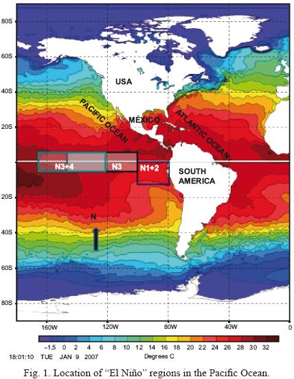
In México, González et al. (2000), have proposed equations through which the runoff behavior in different regions of México can be estimated from the values of the teleconnection indices and from anomalies in the sea surface temperature of three regions associated with the "El Niño" and "La Niña" phenomena (Fig. 1).

In this paper a combination of Fiering and Svanidze methodologies to generate synthetic long term sea temperature records that maintain the statistical characteristics of their historical records is proposed, and is applied in "El Niño" regions. These records could be applied for the simulation of the possible long term variation of runoff in events that are statistically similar to the historical records.

For the study of this phenomenon, daily measurements are taken by the NOAA to get the monthly reports of the sea surface temperatures and their respective anomalies (differences with respect to the average in different ocean regions).

The following is a summary of the classic methodologies used in the generation of synthetic records.

1.1 Background

A problem that arises in climatic and hydrological studies is the insufficiency of measured historic data and incomplete or short–term records. Consequently, it is fundamental to rely upon algorithms through which it is possible to obtain time series records of longer duration than those available, while striving to preserve, as much as possible, the historical statistics of the samples.

Currently, comparisons are made between autoregressive procedures, ARMA(p,q) and artificial neural networks (ANN) or non–parametric methods (nearest–neighbors) (Toth et al., 2000). However, ARMA models will always be a reference parameter to validate results (Abrahart and See, 2000; Tingsanchali and Gautam, 2000).

With these models it is possible to analyze extreme event occurrences, as well as uncertainties, possible climate changes and the strategies to determine even dam operation policies. Such is the case of the Thomas–Fiering model, which has been used to characterize the monthly change in the elevations of water levels in lakes and reservoirs (Somlyódy and Honti, 2005). Furthermore, the study of the conceptual models of the rainfall–runoff processes developed for different climatic scenarios may be nowadays performed with autoregressive models (Liden and Harlin, 2000).

Regarding climate change, remote sensitivity analyses undoubtedly contribute very importantly in these types of studies, and ARMA(p, q) models also have an exceptional applicability in image analysis, particularly to identify changes in diverse hydro–meteorological variables (Piwowar and Ledrew, 2002). However, a problem that arises in climatic and hydrological studies is the insufficiency of measured historic data and incomplete or short–term records. Consequently, it is fundamental to rely upon algorithms that allow the acquisition of time series records of longer duration than those available, while striving to preserve, as much as possible, the historical statistics of the samples.

In general, ARMA(p,q) models have made possible, for over a decade, the study of several autocorrelation functions of the hydro–climatological variables that are used to describe the processes of the hydrologic cycle. Nevertheless, a wide range of improvements to the procedures traditionally used can be found. For example, through empirical models based on daily values series, the ARMA–GARCH/EGARCH schema were created (Karanasos and Kim, 2003). In the case of periodical series, the modified fragment method (Srikanthan and Zhou, 2003), and in general, the Box–Jenkins models (Calzolari et al., 1998; Katsamaki et al., 1998) can be mentioned.

The main problem observed in many of these methods of periodic generation lies in that, as the order of moment progresses, it becomes more difficult to reproduce the corresponding statistics. That is, some of these methods are able to reproduce the average, but not the statistics related to moments of higher order such as the standard deviation or the coefficient of skew. Another limitation of some of these procedures is their inability to reproduce the autocorrelation between the values of the last period of a year (i) with respect to those of the first period of the following year (i+1); this is true for the fragment method of Svanidze (Svanidze, 1980) in its traditional form as is described below. Finally, the majority of the classic models have not been designed to reproduce the cross correlation between the historical values recorded in different sites.

For the reasons stated above, this article proposes an algorithm to generate synthetic series that allows us to reproduce the autocorrelation between the first period of a year (i+1) and the last period of the previous year (i), while preserving the historical statistics of the historical samples, and specially the cross correlations between simultaneous values measured in three rectangular regions nearby the Equator, which are defined by their geographic coordinates and are related to the "El Niño" phenomenon, called Region Niño 1+2 (N1+2), Region Niño 3 (N3) and Region Niño 3+4 (N3+4) (Fig. 1).

2. Methodology

2.1 Svanidze method

A statistical analysis to estimate the distribution function of best fit is performed on the annual total; once such distribution is obtained, m synthetic annual total values are randomly generated with the fitted distribution function. On the other hand, for each recorded year the fraction of each period with respect to the annual total is calculated (Eq. 2); subsequently, m years are randomly selected from the historic record, and their corresponding fractions are multiplied by each random annual total, and a synthetic periodical series of m years is determined.

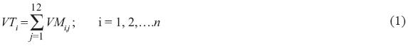
Where:

n number of year for the historical record

m number of years for the generated synthetic series

i counter of years from the historical record (i=1,2,….n)

j counter corresponding to the month under consideration (j=1,2,….12).

VT_i is the annual total of year i for the analyzed variable in the series; VM_i,j is the monthly value j for the year i for the analyzed variable in the series; FVM_i,j is the fraction of the monthly value j for the year i with respect to VT_i (Domínguez et al., 2001).

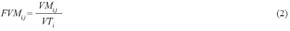
The modification to the Svanidze method consists in applying it to two or more periodical series; it was originally used to generate monthly feed volumes for two reservoirs in series (Domínguez et al., 2001). When two or more series are involved, the annual total is determined for each one, as well as the fragments with respect to the annual total (Eqs. 3 and 4); afterwards, the sum of the annual totals for the n series and the corresponding proportion for each series is calculated; a statistical analysis is performed on the sum of the annual totals to determine the probability distribution function of best fit.

With such distribution m synthetic random values for the sum of the annual totals are generated. On the other hand, m years are randomly selected from the historical record, to consider the fragments corresponding to those n years, as well as the proportion with respect to the sum of the totals. Each random proportion is multiplied by the total sum, which leads to random totals for each series. Finally, these totals are multiplied by the random fragments and with this, the m years of synthetic records for each series are determined.

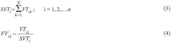
Where SVT_i is the sum, for the N series, of the annual totals for the analyzed variable in year i; VT_i,k is the total value of the analyzed variable in the year i of the series k; FV_i,k is the fraction of the total value of the variable in year i, for the series k with respect to SVT_i ; k is the counter variable corresponding to the series under consideration (k = 1, 2,….N), where N is the total number of series.

This method has the advantage of its relative simplicity, but its main disadvantage is that, due to the way years are selected, the correlation between the last period of a year and the first period of the following year is not preserved. To reduce this deficiency, a record that takes into account the naturally low correlation that exists in the change of seasons may be used (for example, in the case of precipitation or runoff, when moving from dry to flood seasons, so a hydrologic year is defined, having July as the first month and June from next year as the last month instead of January to December).

The sea surface temperatures are characterized by their high autocorrelations from one month to another and the Svanidze modified method has difficulties in reproducing this behavior for the last month of year i to the first month of year i + 1; so, it is necessary to research classical methods and a possible combination of methodologies to overcome this situation.

2.3 Autoregressive moving average models, ARMA(p, q)

These models are mainly applied to annual series; they are a combination of the autoregressive models AR(p) and the moving average models MA(q) (Box and Jenkins, 1976; Salas et al., 1988); the value of p is the number of parameters associated with the autoregressive part while the value of q represents the number of parameters associated with the moving average component. The general representation of ARMA(p,q) models is:

Equation (5)

where η_t is a random variable, calculated in time t; _p,i , i=1,2,…,p are the parameters of the autoregressive component; θ_q,j, j=1,2,…,q are parameters of the moving average component. This method considers data and residuals to be normal and independent. A property of the ARMA(p,q) models is that autocovariances from order 1 to order q depend on the autoregressive parameters fp,i and on the moving averages q_q,j , while for higher orders they are only dependent upon autoregressive parameters (Meddahi, 2003). In the case of discrete series, the autocovariance C of order l (lag) is calculated as:

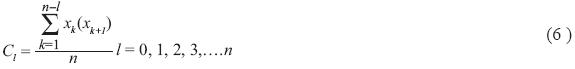
The coefficient of autocorrelation of order one r₁ is obtained through dividing the autocovariance of order one by the autocovariance of order zero, that is:

Other important parameters for the selection of the ARMA model are the coefficients of partial correlation, which can be obtained with the following equations:

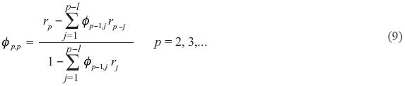
One criterion to select the p and q parameters of the ARMA model is the analysis of the variations of the correlogram (plotting r_l versus l) and in the partial correlogram (_p,p versus p) (Salas et al., 1988).

Another selection procedure is the information criteria of Akaike, that is very frequently used in the definition of hydrograph parameters (Jena and Tiwari, 2006):

where σ² is the variance of the normalized series and C_{x, η} is the covariance between x and η

2.4 Annual Fiering method

The annual Fiering method is the particular case of an ARMA(1,0), commonly known as a Markov model; it assumes that data have a normal distribution, with average µ and variance σ ^_x2; it directly generates synthetic values with a normal distribution function which preserves the average, the variance and the coefficient of autocorrelation of order one for the historical series. The generation model has the following form:

where x_i is the estimated value at instant i; µ is the average of the historical series; σ^_x is the standard deviation of the historical series; r₁ is the coefficient of autocorrelation of order one; t_i is a random number with standard normal distribution (zero average and standard deviation equal to one). Due to the characteristics of the standard normal distribution function, sometimes negative values for t_i may be obtained and this may lead to x_i values that are also negative; both values are utilized to generate the following values, but must be considered null when performing a simulation process.

This method may be employed to generate annual time series that are not normal; for this the variable is transformed so that it has a normal distribution, the generation is performed and finally the de–normalization process is carried out. Nevertheless, since the transformations that are used for normalization (calculation of logarithms, Box–Cox transformations (Kite, 1988)) are not linear, the results obtained are approximations.

2.5 Data analysis

Information of the recorded values of the monthly sea surface temperature (SST) was obtained for the period of 1950 to 2003 in the Regions Niño 1+2, Niño 3 and Niño 3+4 that are located in the Pacific Ocean (Fig. 1); these values were reported by the Climate Prediction Center of the National Weather Service that belongs to the National Oceanic and Atmospheric Administration (NOAA). To identify a possible trend or a cyclical component, the variation in the time of the monthly sea surface temperatures (SST) in each region was analyzed (Figs. 2 a, b and c). The monthly and annual average temperature statistics were calculated; additionally, the autocorrelations between month j+1 and month j as well as the cross correlations of month i of region k with month i of region k+1 (Figs. 3a and b) were obtained.

With the preceding information the Svanidze method could be employed since it is able to reproduce the autocorrelations from a month to another month in the same period of the year, as well as the cross correlations; nonetheless, the Svanidze procedure has problems in maintaining acceptable correlation values between the last period of year i and the first period of year i + 1. To justify the possible use of an ARMA(p, q) model for the annual average data, the total and partial correlogram for each region were determined, with their corresponding confidence intervals (a= 0.05); the respective correlograms are shown in Figs. 4, 5, 6.

In these figures it can be observed that the autocorrelation for the annual values falls practically always within the confidence intervals; this means that the use of an ARMA(p, q) model should not lead to an improvement of results.

3. Results

3.1 Application of Svanidze, modified Svanidze and ARMA–Svanidze methods

The historical statistics and the correlations of the temperatures in the three regions were compared to the results obtained by the application of three methods: the Svanidze method to each region under analysis, the modified Svanidze method (simultaneously considering the three regions) and an ARMA–Svanidze combined form, using an ARMA(2,1) model (selected after applying the information criterion of Akaike) to generate the annual average data and the Svanidze method to consider simultaneously the three regions for the monthly data. The results are shown in Figs. 7 to 11. According to Figs. 7 to 11, it can be observed that the average is adequately reproduced by the three methodologies, (the maximum difference of 0.24% was observed by applying Svanidze to the Region Niño 1+2); regarding the standard deviation the worst method is the ARMA–Svanidze, with maximum differences up to 0.59 in the regions Niño 3 and Niño 3+4; with respect to the coefficient of skew practically all methods present difficulties, mainly in the Region Niño 1+2 where the maximum differences were of 1.87 for the ARMA–Svanidze method, 1.85 for the Svanidze method and 1.37 for modified Svanidze; autocorrelations are adequately reproduced with all the procedures (with maximum differences on the order of 0.10), with the exception of the autocorrelation between the last period of year i and the first period of year i+1, with differences on the order of 0.90 for the three methods. As was expected, the cross correlations were not reproduced by the Svanidze method applied individually to each region whereas with the ARMA–Svanidze and modified Svanidze methods the maximum differences were only of 0.13 and 0.25 respectively.

3.2 Application of Fiering–Svanidze method

Taking into account that autocorrelations do not show a clear cyclical component, it was proposed to use the series corresponding to the sum of the monthly values for the three regions under analysis, its standardization month to month for each year, with the corresponding statistics, and the posterior synthetic generation as if each month were a year, with the assistance of the Annual Fiering method; afterwards, the un–standardization of the series would be performed and finally the random distribution of the monthly percentages for each region would be carried out through the Svanidze method.

The monthly series was formed by the sum, month to month, of the 54 recorded years in the three regions under analysis.

Where T ^k_i,j is the measured temperature of the month j of year i in region k; Ts_i,,j is the sum of the measured temperatures in month j of year i for the three regions.

For this summed record of n years the average and the standard deviation of each month were calculated.

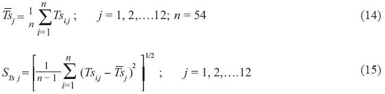
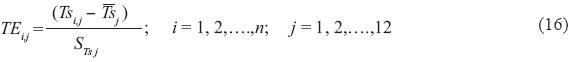
To remove the cyclical component of the average and the standard deviation, the summed record was standardized subtracting the average and dividing by the standard deviation of each month.

Next, a record TC_k was built, in only one column, placing historical year 1 through historical year 54, one after another, the values for months 1 through 12.

Once the autocorrelogram and the partial correlogram of the new series were obtained, it was observed that it can be approximated with an AR(1) model or the equivalent Fiering method.

The Fiering method was then applied to generate ten synthetic monthly series of the same size as the historical record (54 years). It was verified that the obtained series had an average of zero and a standard deviation approximately equal to one.

The obtained series corresponded to the synthetic values standardized from the sum of the regions, so it was necessary to un–standardize it using the average and the standard deviation of each month of the historical series (Eqs. 14 and 15).

The results of the historical and synthetic statistics for the summed region are presented in Figure 12 which shows that, with the exception of the coefficient of skew, statistics are adequately reproduced.

On the other hand, for each month and year of the historical record the fraction for each region with respect to the historical sum was available:

A random selection of an historical year i and therefore of its fractions FT_i,j^k was performed to distribute, in each one of the regions, the generated summed record, in a similar way to the process of the modified Svanidze method. The results of the statistics for each region compared against the historical are shown on Figures 13 to 17.

In Figures 13 and 14 it is observed that the average and the standard deviation are well reproduced, with maximum differences in the averages up to 1.73% , for the Region Niño 1+2, 1.76% for the Region Niño 3 and 1.88% for the Region Niño 3+4; in the standard deviation there are differences up to 0.57 in the Region Niño 3+4. The coefficient of skew is reproduced at least in its tendency (Fig. 15), but with maximum differences up to 1.83 for the Region Niño 1+2.

Concerning Figure 16, results are encouraging inasmuch as the combination of the Fiering and Svanidze methods, as has heretofore been proposed, overcomes the deficiencies that appeared in previous procedures (Svanidze and the ARMA–Svanidze combination) due to the good concordance between the coefficients of correlation of the first month of the subsequent year with respect to the last month of the preceding year, with a maximum difference of 0.10 for the Region Niño 1+2 (February with January), 0.14 for the Niño 3 (April with March) and 0.12 for the Region Niño 3+4 (June with May). The behavior of the cross correlations is reproduced as well (Fig. 17), with a maximum difference 0.27 of Region Niño 1+2 with Region Niño 3+4.

Finally, the lagged correlation of three consecutive months was estimated for the Fiering–Svanidze method for the three regions, in order to analyze some results directly related with the persistence during several months. A good agreement with the historical coefficients was observed. This is shown in Figure 18. In addition the average frequency between two "El Niño" and two "La Niña" episodes resulted of 4.9 and 2.1 years respectively, in comparison with the frequency of 4.9 and 3.6 years for the historical record.

Sea surface temperatures determine in part runoff conditions in vast continental zones. Such is the case for the sea surface temperatures in the regions called Region Niño 1+2, Region Niño 3 and Region Niño 3 + 4, which strongly influence runoff in the Pacific basins of México. Historical temperature series are, however, limited, so it becomes convenient to generate synthetic records of longer duration from which it will be possible to visualize scenarios that have not appeared or have not been measured.

Synthetic records must preserve statistical characteristics of the historical series, which becomes difficult in the case study fundamentally because the monthly autocorrelations are maintained above 0.75 throughout the year and also because the cross correlations between regions are high as well.

The autocorrelations between annual average sea surface temperatures in the analyzed regions show that the application of an AR(1) model is justified, due to their scarce autocorrelation (see Figs. 4, 5, 6). Nevertheless, the information criterion of Akaike reports that good results would be obtained with an ARMA(2,1) model.

In conformance with these results, records were generated by utilizing the Svanidze method, the modified Svanidze method, and a combination of the ARMA(2,1) model for annual data and the Svanidze method to distribute between the regions and months.

The results show that the behavior pattern of the average and the standard deviation were reproduced (see Figs. 8 and 9), as well as the coefficient of skew to a lesser degree (Fig. 10), but the coefficients of autocorrelation were not reproduced for the last month of year i with respect to the first month of the following year (Fig. 11). The cross correlations were preserved with the Modified Svanidze method and with the ARMA–Svanidze, while this was not accomplished by Svanidze applied independently to each region (Fig. 12). In general terms and due to the above considerations, we consider that the Modified Svanidze method is the one that produces the best response for the statistics and the cross correlations in the analyzed monthly data series; however, its deficiency to reproduce the correlation of the last period of year i and the first period of year i + 1 persists.

The final proposal named Fiering–Svanidze consisted in generating the monthly data from the summed record of the three stations as if they were annual and applying the Fiering method. The generated values were later distributed in each region with the random procedure employed by Svanidze. In this way, in addition to adequately reproducing the statistics of each region and the cross correlations between regions, the coefficients of autocorrelation in the three analyzed regions were reproduced as well (Figures 16 and 17).

The generation of synthetic samples using this last proposed combination of methodologies allowed us to analyze the possible long term behavior of the values for the sea surface temperature and to model "El Niño" or "La Niña" episodes which determine in part the hydrological behavior of the Pacific basins in Mexico.

References

Abrahart R. R. and L. See, 2000. Comparing neural network and autoregressive moving average techniques for the provision of continuous river flow forecasts in two contrasting catchments, Hydrological Processes, Vol. 14, pp. 2157–2172.         [ Links ]

Box G. E. P. and G. M. Jenkins, 1976. Time series analysis, forecasting and control. 2nd ed. San Francisco, CA. Holden–Day.         [ Links ]

Calzolari G., F. Di Iorio and G. Fiorentini, 1998. Control variances reduction in indirect inference: Interest rate models un continuous time. Econometrics Journal, 1, C100–112.         [ Links ]

Domínguez R., M. G. Fuentes and M. L. Arganis, 2001. Procedimiento para generar muestras sintéticas de series periódicas mensuales a través del método de Svanidze modificado aplicado a los datos de las presas La Angostura y Malpaso. Series del Instituto de Ingeniería, UNAM, Serie Blanca CI–19. Agosto.         [ Links ]

Elfeki A., 2006. Reducing concentration uncertainty using the coupled Markov chain approach, J. Hydrol. 317, 1–16.         [ Links ]

González V. F .J., V. Franco, G .E. Fuentes M. and M. L. Arganis J. 2000, "Análisis comparativo entre los escurrimientos pronosticados y registrados en 1999 en las regiones Pacífico Noroeste, Norte, Centro, Pacífico Sur y Golfo de la República Mexicana considerando que estuvo presente el fenómeno "La Niña" y Predicción de escurrimientos en dichas regiones del país en los periodos primavera–verano y otoño–invierno de 2000", Instituto de Ingeniería, UNAM, Informe final para el Fideicomiso de Riesgo Compartido, Banco Nacional de Crédito Rural, S. A., Secretaría de Agricultura, Ganadería y Desarrollo Rural. Noviembre.         [ Links ]

Hongbing S. and D. Furbish, 1997. Annual precipitation and river discharges in Florida in response to El Niño– and La Niña– sea surface temperature anomalies, J. Hydrol. 199, 74–87.         [ Links ]

Jena S. and K. Tiwari, 2006. Modeling synthetic unit hydrograph parameters of watersheds, J. Hydrol. 319, 1–14.         [ Links ]

Karanasos M. and J. Kim, 2003. Moments of the ARMA–EGARCH model. Econometrics Journal6, 146–166.         [ Links ]

Katsamaki A., S. Williems and E. Diamadopoulos, 1998. Time series analysis of municipal solid waste generation rates. J. Environmental Engineering 24, 178–183.         [ Links ]

Kite G. W., 1988. Frequency and risk analyses in hydrology, Water Resources Publication. USA, 257 pp.         [ Links ]

Liden R. and J. Harlin, 2000. Analysis of conceptual rainfall–runoff modelling performance in different climates. J. Hydrol. 238, 231–274.         [ Links ]

Meddahi, N., 2003. ARMA representation of integrated and realized variances. Econometrics Journal 6, 335–356.         [ Links ]

NOAA, 2005. National Oceanic and Atmospheric Administration, Comunicado de prensa 10 de febrero de 2005 en Internet: http://usinfo.state.gov/esp/Archive/2005/Feb/16–798645.html.         [ Links ]

Piwowar J. M. and F. E. Ledrew, 2002. ARMA time series modeling of remote sensing imagery: a new approach for climate studies. Int. J. Remote Sens. 23, 5225–5248.         [ Links ]

Ropelewski C. F. and M. S. Halpert. North American precipitation and temperature patterns associated with the El Niño/Southern Oscilation (ENSO). Mon. Wea. Rev. 114, 2352–2362.         [ Links ]

Salas J. D., J. W. Delleur, V. Yevjevich and W. L. Lane, 1988. Applied modeling of hydrological time series. Water Resources Publications, USA.         [ Links ]

Sanso B. and L. Guenni, 1999. A stochastic model for tropical rainfall at a single location, J. Hydrol. 214, 64–73.         [ Links ]

Shukla J. and J. M. Wallace, 1983. Numerical simulation of the atmospheric response to equatorial Pacific sea surface temperature anomalies. J. Atmos. Sci. 40, 1613–1630.         [ Links ]

Somlyódy L. and M. Honti, 2005. The case of Lake Balaton: how can we exercise precaution? Water Sci. Technol. 52, 195–203.         [ Links ]

Srikanthan R. and S. Zhou, 2003. Stochastic Generation of Climate Data, Technical Report. Report03/12, Cooperative Research Centre for Catchment Hydrology, Australia, November.         [ Links ]

Svanidze G. G., 1980. Mathematical Modeling of Hydrologic Series, Water Resources Publications, USA.         [ Links ]

Thyer M. and G. Kuczera, 2003a. A hidden Markov model for modeling long–term persistence in multi–site rainfall time series 1. Real data analysis. J. Hydrol. 275, 12–26.         [ Links ]

Thyer M. and G. Kuczera, 2003b. A hidden Markov model for modelling long–term persistence in multi–site rainfall time series 2. Real data analysis. J. Hydrol. 275, 27–48.         [ Links ]

Tingsanchali T. and M. Raj Gautam, 2000. Application of tank, NAM, ARMA and neural network models to flood forecasting, Hydrological Processes 14, 2473–2487.         [ Links ]

Toth E., A. Brath and A. Montanari, 2000. Comparison of short–term rainfall prediction models for real–time flood forecasting, J. Hydrol. 239, 132–147.         [ Links ]