Oscar De la Torre Torres**

** Facultad de Contaduría y Ciencias Administrativas, Universidad Michoacana de San Nicolás de Hidalgo. Correo electrónico: oscar.delatorre@uam.es.

Fecha de recepción: 10/09/2012.
Fecha de aprobación: 23/04/2013.

This paper presents the usefulness of an active portfolio management process with orthogonal GARCH (OGARCH) matrixes in order to achieve a 7.5% actuarial target return in defined benefit pension funds such as the Dirección de Pensiones Civiles del Estado de Michoacán. To prove this, four discrete event simulations were performed using, in the first scenario, a passive portfolio management process with a target position rebalancing discipline and, in the other three, an active portfolio management with a range portfolio rebalancing one. In these last three simulations, a constant covariance, a Gaussian distribution OGARCH and a Student's t-distribution OGARCH covariance matrix were used. The attained results suggest that the Student's t-distribution OGARCH matrix is the most suitable for the investment process.

Keywords: portfolio choice, asset pricing, financial forecasting and simulation, hypothesis testing.

JEL classification: C12, G11, G12, G17.

Resumen

En el presente artículo se prueba la utilidad de un proceso de administración activa de portafolios con matrices de covarianzas GARCH ortogonal (OGARCH) en la reserva técnica de fondos de pensiones de beneficio definido, como es el caso de la Dirección de Pensiones Civiles del Estado de Michoacán. Esto, para lograr el objetivo de un rendimiento anual de 7.5% establecido en su estudio actuarial. Para demostrarlo, se realizaron cuatro simulaciones de eventos discretos en donde se ejecutó, en un escenario, un proceso de administración pasiva de portafolios con una disciplina de rebalanceo tipo posición objetivo, y en otros tres, uno de administración activa de tipo rebalanceo por rangos. En los últimos tres casos se empleó una matriz de covarianzas constantes, una OGARCH con función de verosimilitud gaussiana y una OGARCH con función t de Student, respectivamente, demostrando con los resultados observados la conveniencia de utilizar esta última en el proceso de inversión.

Palabras clave: selección de portafolios, valuación de activos, pronósticos y simulaciones financieras, pruebas de hipótesis.

Clasificación JEL: C12, G11, G12, G17.

One of the main fiscal and financial needs in the medium- and long-term in Mexico is the proper financial management and funding of the defined benefit pension funds of the public servants in each state in the country. Several proposals have been made by academics or by the Presidency of Mexico such as either structural or parametric reforms in their financial planning. The migration from a defined benefit plan to a defined contribution one, the renegotiation of the future contract liabilities with unions or the change in the investment regime are among the most common ones. A detailed review of the main reform proposals is outside the scope of the present paper. A very straightforward review is given by the Instituto Mexicano de Ejecutivos de Finanzas (IMEF, 2006), or Mexican Financial Executives Institute, for any interested reader. The aim of the present paper is to present the simulation results of one of the potential solutions that the pension fund owned by the public servants of the state of Michoacan¹ wants to test: An active portfolio investment process with OGARCH covariance matrixes used to achieve an actuarial annual target return of 7.5% in their “technical reserve”.² These results are presented in order to show the usefulness of the active portfolio management³ process with OGARCH covariance matrixes in defined benefit pension funds with a stream of liabilities like the observed ones in this case.

One of the main concerns is to test the attained results with the historical asset allocation in the six different markets presented in the investment policy statement (IPS) show in Table 1. For this purpose, a benchmark that incorporates this asset allocation and its limits is also given in the table along with the target positions.

Now that the main target of the present paper has been mentioned, it is necessary to talk about the optimizers used in the context of a portfolio management algorithm devised to test the suitability of the proposed investment process. Since the seminal work of Markowitz (1952) several alternative optimal portfolio selection models have been the standard in asset or asset and liability management activities for institutional investors such as pension funds. The first developments in portfolio selection models focused on a “buy and hold” rationale, given the optimal investment proportions determined with the investor’s utility function (usually a quadratic one) and a specific time horizon. This type of investment strategy is part of a group of practices known nowadays as passive portfolio management. With the advent of the Markowitz-Tobin-Sharpe-Lintner model (MTSL) (Markowitz, 1987, p. 5) and the assumption of aggregate optimality due to homogeneous expectations among investors (Samuelson, 1965) that leads to the concept of market equilibrium (Sharpe, 1963; Lintner, 1965), the stock market indexes where used not only as a statistical measure of the aggregate investor behavior but also as a proxy of the market portfolio, which is a key concept in the main asset pricing models.

Due to several economical, financial, and behavioral circumstances, the aggregate optimality (as a proxy definition of equilibrium in financial markets) is not observable in the short-term, suggesting the preference of the active portfolio management practice. This situation has improved with the development, in the decade of 1950, of time series analysis through the seminal work of Box, Jenkins and Reinsel (2008) for the expected returns and later with the proposals of Engle (1982) and Bollerslev (1986) for the short term volatility forecast. With these quantitative developments, the portfolio management theory had a positive and practical advance in order to explore and exploit short-term price differentials in respect to equilibrium ones, leading to support the active management practice. Several researches have been published in order to test active portfolio management against the passive approach in the mutual fund industry with cases such as Daniel et al. (1997) and Ennis (2005) who found, through the mutual fund comparison against a stock index after management fees, that active management couldn’t lead to a better performance than the one obtained from a passive management practice, such as index tracking or enhanced index tracking.⁴

In some cases (such as index tracking) the passive management strategy could be implemented by following a target positions (TP) rebalancing discipline where the portfolio position is rebalanced to the benchmark position (W_bmk). On the contrary, active management practice, that seek to outperform a benchmark or a market index, could be executed with two rebalancing disciplines (among the most used ones) known as percentage portfolio rebalancing or range portfolio rebalancing (RPR). The former is a rebalancing method executed at periodically specified time intervals where the portfolio manager adjusts the investment positions to a range of ±x% from a target optimal position W_bmk; the latter consist of discretionary investment proportions that must follow upper and lower asset or market type limits, stated in an IPS such as the one presented in Table 1.

From the several strategies widely used as rebalancing disciplines in the portfolio management practices and from the aforementioned ones, the pension fund of interest wants to test a RPR discipline using the IPS shown in Table 1 as in a relatively discretional manner in different types of assets allowed in the IPS.

In order to test whether a TP passive portfolio management strategy or an active RPR one is more suitable to the fund, four discrete event simulations were performed. One for the passive portfolio management case with a TP regime and three for the RPR active portfolio management that use three different covariance matrixes: 1) an orthogonal generalized autoregressive conditional heteroskedasticity (OGARCH) with Gaussian log likelihood function, 2) an OGARCH with a Student's t-distribution (or just Student's t) or 3) a constant covariance likelihood.

Once the target of the present paper has been established (to test the use of active portfolio with OGARCH matrixes in the investment management of this pension fund and similar ones) the results will be presented as follows: in section i a brief explanation of the Markowitz-Tobin-Sharpe-Lintner model is given along with the need and review of the OGARCH covariance matrix model. Following this, the assumptions and general structure of the algorithm used in the four discrete event simulations are presented along with a review of the attained results. Once this is done, the document ends with the concluding remarks.

1. The Markowitz-Tobin-Sharpe-Lintner portfolio selection model

The first quantitative approach or optimizer for the portfolio selection problem is proposed by Markowitz (1952) where he states that the investor must perform a rational⁵ mean return-variance portfolio selection taken from an efficient set ξ determined from a bigger set Ξ of portfolios known as the investment set where ξ ⊂ Ξ.

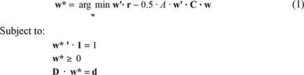
In order to select the optimal portfolio given an n x 1 investment proportion vector w, a n x n covariance matrix C, an n x 1 expected return vector r = [E (r_i) ... E (r_n)]', an l x n asset or market grouping matrix D; a l x 1 minimum or maximum limits vector d established in the IPS (such as the one described in Table 1), and also a risk aversion measure a, the next quadratic program can be solved:

As noted, the optimal portfolios selection is made by assuming a quadratic expected utility function, following the proposal of Levy and Markowitz (1979) of a second order Taylor expansion around the portfolio expected return E_P. One of the main drawbacks of the optimal selection model⁶ in equation (1) is that it cannot include the investment proportion in a risk free asset rf due to the theoretical (statistical) interpretation of cov (rf,r_i.) = 0, σ²(rf) = 0 that leads to a singular matrix C when (1) is solved. In order to sort this situation and as an explanation to the investor’s speculative motivations proposed by Keynes, Tobin (1958) presented his theory known as Liquidity preference as behavior towards risk,⁷ that allowed the development of a quantitative model for the optimal portfolio selection where the optimal selection is now conceived as a linear combination of rf and a risky portfolio given by w*. This selection is performed as two step problem that starts with the first solution given by:

The second step is given by the solution of the proportion in the total investment budget ω in w* and the proportion (1-ω) in rf by using a utility function such as equation (2) in the next expression:⁸

The portfolio selection model in equation (4) is known as the Markowitz-Tobin-Sharpe-Lintner model or MTSL (Markowitz, 1987, p. 5) and is one of the most widely used in the portfolio management industry (as is the case in the present paper) because it incorporates a risk free asset in the asset allocation step. Although the rationale of the MTSL is a very straightforward one, its main drawback is in the calculation of r and C due to the presence of estimation errors; its computational inefficiency, and also the presence of volatility and correlation clustering. As a potential solution for the computational efficiency problem, Sharpe (1963) proposed an alternative calculation of such parameters that later lead him to the proposal of the capital asset pricing model (CAPM) (Sharpe, 1964).⁹ This valuation model is the theoretical fundation of several heuristics procedures and alternative valuation models that have, as a central concept, the covariace of assets now proxied through the covariance with a common factor or set of factors. Although the CAPM is a straightforward rationale for asset pricing and by setting aside the theoretical critiques made towards it, the presence of volatility and correlation clustering and the potential presence of estimation errors are one of its main drawbacks as is the general case of the most used models of modern portfolio theory. Therefore, because of practical issues, such as the determination of the most suitable nonstandard CAPM, we will adopt a pure mean-variance framework that will lead us to choose the MTSL model as the optimizer for the asset allocation step in the portfolio management process.

Once the motivation for the use of the MTSL model is mentioned and following Best and Grauer (1991) that suggest that the optimal portfolio selection is sensitive to the sample magnitude observed in r and C, the aim of the present paper is to test the use, in defined benefit pension funds such as the Dirección de Pensiones Civiles del Estado de Michoacán, of an active portfolio management process using Orthogonal GARCH (OGARCH) matrixes in order to incorporate the effect of the volatility and correlation clustering in the asset allocation step. Given this, it is necessary to review this multivariate volatility model.

2. The Orthogonal GARCH model (OGARCH) for the calculation of the covariance matrix

With the earliest proposals of Engle (1982) and Bollerslev (1986), the calculation of short term volatilities that incorporate the volatility clustering effect allowed the financial practice to perform more appropriate risk level forecasts. The univariate GARCH (p,q) model is described by the following expression:

As a starting point for the present paper, the GARCH (p,q) model departs from the assumption that the returns vector r_i of the i^th asset is either¹⁰ leading to the more general assumption of multivariate elliptic probability functions in the set of returns time series X = [r₁, ..., r_i]. With this assumption, the log likelihood problem can be solved through two functions. If 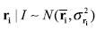the vector of parameters θ_i =[ K, [β_i], [γ_i]] leads to¹¹ σ²_t = σ²_t (θ_i) in (5) and the optimal set of parameters 0* is given with the solution of the next optimization problem:

When , the solution is given by the next log likelihood function maximization:¹²

For the multivariate case, the first proposal is the one made by Bollerslev (1990) that starts with the use of a constant correlation matrix H and a diagonal matrix S with a diagonal defined by univariate GARCH variances:

C_t = S_t· H_t· S_t (8)

Even though the relative computational efficiency, the model does not take into account the correlation clustering effect. A proposal that solved this situation was formulated by Engle and Kroner (1993) but, in some cases, an observable computer capacity is needed given the log likelihood maximization problem inherent to it. As a solution for this situation, a model known as Orthogonal GARCH (OGARCH (p,q) ) or simply OGARCH is proposed in Alexander and Chibumba (1996), Alexander (2001) and Van der Weide (2002). This model departs from the spectral decomposition of a constant¹³ covariance matrix C_c that leads to the definition of an n x n matrix of eigenvectors E and a n x n spectrum Λ:

C_c = E· Λ · E (9)

The computational efficiency of the OGARCH model is based in the variance (eigenvalues) of the principal components (P = X· E = [p₁ ..., p_i]) given in the diagonal elements of Λ. Once this matrix is defined, a selection of principal components, eigenvalues and eigenvectors is made by sorting the eigenvectors and principal components from the highest (h) to the lowest eigenvalue. Once this is done, the next selection criteria is applied, given a total variance explanation level previously fixed :

With the definition of Λ* the calculation of a univariate GARCH volatility is made in each principal component in P* by using the log likelihood functions given either in equations (6) or (7). This will lead to the definition of a GARCH spectrum Ω and to the next matrix composition of the expected OGARCH covariance matrix:

Now that the calculation of the MTSL model and the OGARCH covariance matrix have been reviewed as parts of the optimizer for portfolio management process to be tested, the assumptions of the four discrete event simulations Appendix 2.

II. The discrete event simulations performed

1. Statistical parameters, theoretical assumptions, and practical implications in each simulation

Given a time window from January 2, 2002 to December 31, 2010, 470 weekly interval simulations were performed for each simulated portfolio, departing from a base value of 100 on December 29, 2000 in each of the benchmarks presented in Table 1 as financial assets.¹⁴ Given this, it is assumed that these values represent the behavior of zero tracking error Exchange-Traded Funds (ETF’s) invested in each benchmark.

These benchmarks were valued in Mexican pesos (MXN) and their value incorporate currency impact. The length in each asset or market returns time series (r_i) is T = 52 weeks length. A quantitative analysis algorithm that performed the entire portfolio selection process (analysis, rebalancing, and mark to market valuation) was programmed in MATLAB and, among the most relevant ones, follows the next assumptions and parameters:

1. The theoretical¹⁵ starting value of the four simulated portfolios is MXN 10 000 000.00, an amount that is also affected in value, along with the entire portfolio value, by the inflows and outflows observed in the pension fund described in Appendix 1.

2. The financial data sources are Bloomberg™, Reuters™ and InfoselMR.

]]> 3. In order to incorporate the impact of financial costs, a 0.25% fee is assumed in each trade either in the ETF’s or in the foreign exchange market (FX ), noting that even though a institutional investor such as the Dirección de Pensiones Civiles del Estado de Michoacán has access to a lower transaction cost, the one listed above will be used in order to measure a higher impact in the final turnover results. The presented fee is for an average individual retail client, noting that almost all the brokerage firms in Mexico and their branches in the United States handle this financial cost.

4. The risk free asset rf used is the weekly secondary market curve rate of the 28 day maturity Certificados de la Tesorería (CETES) (Mexican treasury certificates), a rate that is published by the Banco de México (2012).

5. Only a MXN bank account and two investment contracts (one in USD –dollars of United States– and another in MXN) will be used. When a foreign asset position (USD valued) is sold, the amount is turned into Mexican pesos by selling USD using the current FX rate. When the opposite happens, the USD amount is funded from the Mexican bank account.

6. Expected values in the return vector r are given by the next expression:

In order to calculate the OGARCH matrix with equation (11) either by using (6) or (7) as the log likelihood function, the algorithm selected the best GARCH (p,q) model for each principal component by using different ARCH lag terms truncated at five and different GARCH lag terms truncated at two. The fitness of the best GARCH model in each principal component was determined with the Bayesian information criterion of Schwarz (1978).

For the passive management (TP) portfolio simulation, the main assumption is that all the investment balance is allocated in the risky asset given by the benchmark asset allocation (w*=w_bmk). In order to make the rebalancing from the actual investment proportion to the target one, a 0.25% financial cost was also incorporated and the algorithm shown in Figure 1 was used¹⁶ for this purpose. In order to perform the three discrete event simulations in the active portfolio management scenario, the algorithm in Figure 2 was also used.

In order to compare the attained results, the four historical simulated portfolios were valued in a base 100 value on January 2, 2002.

2. Observed results in the performed simulations

The historical value of the simulated portfolios and their accumulated turnover is presented in Chart 1 and resumed in Table 2. It is shown that the four simulated portfolios and the benchmark had a better performance than a theoretical financial asset that paid the 7.5% target return (shown as a light area). As shown, the simulated portfolios using the OGARCH covariance matrixes lead to a superior turnover than the benchmark, the passively managed and the constant parameter covariance matrix portfolios.

In order to confirm this result and following the portfolio management performance evaluation practices, a quality chart of the difference between the observed weekly return of each simulated portfolio and the benchmark’s is presented in Chart 2. As can be noted in the OGARCH portfolios, the difference between the benchmark and this two specific cases lead to positive alpha, suggesting a better performance if an OGARCH matrix is used in the active portfolio management.

A more detailed examination of the attained results during the four simulations is presented in Chart 3, were the historical allocation between the risk free asset rf and the risky portfolio w* can be observed. The reader can note that the portfolios simulated with an OGARCH covariance matrix (specifically the Student's t one) were more sensitive in the risk free asset investment proportion during the dates where the financial crisis was acute (e.g., the Lehman Brothers Chapter 11 filling in the September-October 2008 period). This is because the volatility and correlation clustering effect¹⁷ was measured more appropriately in this case, leading to a higher concentration in the risk free asset for longer time periods in comparison to the other two cases.

Another perspective of the attained results is given with entire historical asset allocation in Chart 4. In the case of the two OGARCH covariance matrixes portfolios, the optimizer manages the investment more appropriately in risky markets such as the Mexican equity (IPC) or the foreign equities modeled with the MSCI Global Gross equity. This historical behavior is resumed in the box plots of Chart 5 where the reader can observe a summary of the different investment levels in each asset type in each portfolio.

With the observed results in Chart 4 and Chart 5, two questions could be stated: Given the historical asset allocation resumed in Chart 5, does this higher active investment proportions in riskier assets lead to a better performance in the OGARCH simulated portfolios?, and did the financial, political and economic events have an impact in the behavior of the simulated portfolios, leading to a better performance with the use of OGARCH matrixes? In order to answer the first question, Chart 6 presents the historical performance of the six markets in the IPS of Table 1 along with the historical accumulated value of 7.5% annual target rate (light area).

As noted, the best performers were the Mexican equity, Mexican sovereign bonds, and Mexican treasuries markets. If this historical performance is compared with the investment proportions of Chart 4 and Chart 5, it can be noted that the highest investment proportions in the OGARCH models is in this three markets. By inspecting with more detail Chart 4, the performance of the portfolio analysis in the OGARCH cases suggest a more sensitive asset allocation in presence of volatility and correlation clustering, i.e., these two portfolios were better diversified in the most uncertain moments in the financial markets.

The second question, “Did the financial, political and economic events have an impact in the behavior of the simulated portfolios, leading to a better performance with the use of OGARCH matrixes?” is answered in Chart 7 were the historical behavior of the four actively managed portfolios is compared against the financial and economic events shown in Chart 6. The most observable period of this chart is when Lehman Brothers filed for a Chapter 11 application. During this time period, the volatility and correlation clustering effect was more observable.¹⁸ For this reason, and because of their statistical properties, the OGARCH portfolios had a softer behavior than the benchmark and the constant parameter covariance matrix portfolio when the financial crisis was acute.

Once that the fitness of the OGARCH matrixes for the active portfolio management is proved, it can be noted that there’s practically no difference in the selection of the most appropriate log likelihood function (Gaussian or Student's t) so the question of which one of both is preferable must be answered. In order to do so, the Sharpe ratio or SR (a measure of the risk-return trade off) (Sharpe, 1966), was calculated and the historical results are presented in Chart 8. In the lower panels, the historical SR is presented along with a box plot comparison of its historical value.

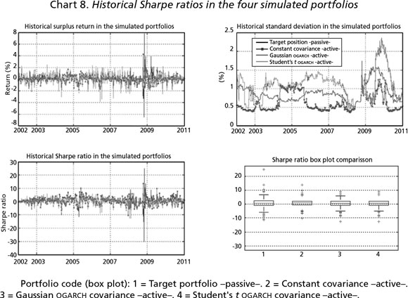
Table 3 presents the results of a one-way ANOVA (analysis of variance) test in the historical SR levels, suggesting that the use of OGARCH matrixes leads to a better and more stable risk-return tradeoff than the passive and constant covariance matrix portfolios. Even though this result can be stated with the OGARCH portfolios against the other two cases, it can also be noted in the lower right panel of Chart 8 that the difference between the Gaussian and Student's t OGARCH portfolio is negligible and leads to no statistical conclusion. Therefore the use of a Student's t OGARCH matrix is suggested by observing, theoretically speaking, that this log likelihood function is more suitable to fit sample multivariate distributions and to model fat-tailed distributions in a better fashion, leaving this last statement to further research.

Concluding remarks

Given the IPS of Table 1 and from the results observed in the four simulations performed, it is concluded that the range portfolio rebalancing discipline with OGARCH matrixes in an active portfolio management process is the most suitable for the technical reserve of the Dirección de Pensiones Civiles del Estado de Michoacán and similar defined benefit pension funds. This conclusion is supported by the achievement of the 7.5% actuarial target return and by a higher turnover than the benchmark, the passively managed and the constant covariance matrix portfolios.

As noted in the attained results, the use of OGARCH matrixes leads to a more suitable asset allocation in the simulated portfolios. This remark is confirmed by the fact that the MTSL model used in these scenarios managed, in a better fashion, the investment proportion in the risk free asset rf given the presence of volatility and correlation clustering.

Also, as noted in a historical analysis as the ones performed in Chart 6 and Chart 7, the actively managed OGARCH portfolios were more sensitive to the influence of financial, political, and economical events. This is so by observing, in these two cases and compared with the benchmark, a softer portfolio performance and a more appropriate asset allocation in the risky asset w* during critical time periods. As a final remark, the use of a Student's t-distribution function is suggested for the calculation of the OGARCH matrixes. This is because even though there’s no statistical difference in the results observed in the accumulated turnover and risk-return trade off of the two OGARCH simulated portfolios, the Student's t-distribution function is more suitable, in theoretical terms, to fit sample data and to model fat-tailed distributions, leaving the probe of this last statement to further research.

References

Alexander, C. (2001). Orthogonal GARCH. In: Carol Alexander (ed.). Mastering Risk, 2. London: FT-Prentice Hall, pp. 21-38.         [ Links ]

Alexander, C. and Chibumba, A. (1996). Multivariate Orthogonal Factor GARCH”. Working paper, University of Sussex Discussion Papers in Mathematics.         [ Links ]

Banco de México (2012). Vector de Precios de Títulos Gubernamentales. [online] Available at: http://www.banxico.org.mx/portalesEspecializados/tasas [Accessed 3 February 2012]         [ Links ].

Best, M. and Grauer, R. (1991). On the Sensitivity of Mean-Variance-Efficient Portfolios to Changes in Asset Means: Some Analytical and Computational Results. The Review of Financial Studies, 4(2), pp. 315-342.         [ Links ]

Bollerslev, T. (1986). Generalized Autorregresive Conditional Hetersoskedasticity. Journal of econometrics, (31), pp. 307-327.         [ Links ]

---------- (1987). A Conditionally Heteroskedastic Time Series Model for Speculative Prices and Rates of Return. Review of Economics and Statistics, 69(3), pp. 542-547.         [ Links ]

---------- (1990). Modelling the Coherence in Short-Run Nominal Exchange Rates: A Multivariate Generalized ARCH Model. Review of Economics and Statistics, 72 (3), pp. 498-505.         [ Links ]

Box, G., Jenkins, G. and Reinsel, G. (2008). Time Series Analysis Forecasting and Control. Hoboken: John Wiley & Sons Inc.         [ Links ]

Chow, G., Jacquier, E., Kritzman, M. and Lowry, K. (1999). Optimal Portfolios in Good Times and Bad. Financial Analysts Journal, 55(3), pp. 65-74.         [ Links ]

Daniel, K., Grinblatt, M., Titman, S. and Wermers, R. (1997). Measuring Mutual Fund Performance with Characteristic-Based Benchmarks. The Journal of Finance, 52(3), pp. 1035-1058.         [ Links ]

Engle, R. (1982). Autoregressive Conditional Heteroscedasticity with Estimates of the Variance of United Kingdom Inflation. Econometrica, 50(4), pp. 987-1007.         [ Links ]

Engle, R. and Kroner, K. (1993). Multivariate Simultaneous Generalized ARCH. Econometric Theory, 11(1), pp. 122-150.         [ Links ]

Ennis, R. (2005). Are Active Management Fees Too High? Financial Analysts Journal, 61(5), pp. 44-51.         [ Links ]

IMEF (2006). Sistemas de pensiones en México -perspectivas financieras y posibles Soluciones-. México: Instituto Mexicano de Ejecutivos de Finanzas, AC.         [ Links ]

Levy, H. and Markowitz, H. (1979). Approximating Expected Utility by a Function of Mean and Variance. The American Economic Review, 69(3), pp. 308-317.         [ Links ]

Lintner, J. (1965). The Valuation of Risk Assets and the Selection of Risky Investments in Stock Portfolios and Capital Budgets. The Review of Economics and Statistics, 47(1), pp. 13-37.         [ Links ]

Markowitz, H. (1952). Portfolio Selection. The Journal of Finance, 7(1), pp. 77-91.         [ Links ]

---------- (1987). Mean-Variance Analysis in Portfolio Choice and Capital Markets. New York: John Wiley & Sons Inc.         [ Links ]

Samuelson, P. (1965). Proof That Properly Anticipated Prices Fluctuate Randomly. Industrial Management Review, 6(2), pp. 41-49.         [ Links ]

Schwarz, G. (1978). Estimating the Dimension of a Model. The Annals of Statistics. 6(2), pp. 461-464.         [ Links ]

Sharpe, W. (1963). A Simplified Model for Portfolio Analysis. Management Science, 9(2), pp. 277-293.         [ Links ]

---------- (1966). Mutual Fund Performance. The Journal of Business, 39(1), pp. 119-138.         [ Links ]

---------- (1964). “Capital Asset Prices: A Theory of Market Equilibrium Under Conditions of Risk. The Journal of Finance, 19(3), pp. 425-442.         [ Links ]

Smith, V. (1962). An Experimental Study of Competitive Market Behavior. The Journal of Political Economy, 70(2), pp. 111-137.         [ Links ]

Tobin, J. (1958). Liquidity Preference as Behavior Toward Risk. Review of Economic Studies, 25(1), pp. 65-86.         [ Links ]

Van der Weide, R. (2002). GO-GARCH: a Multivariate Generalized Orthogonal GARCH Model. Journal of Applied Econometrics, 17(5), pp. 549-564.         [ Links ]

Notes

* The author wants to thank Rosa Hilda Posadas and Antonio Delgado García, former general managers of Dirección de Pensiones Civiles del Estado de Michoacán and Gustavo Arias, the actual finance director, for the support and interest given to the present paper. Any grammar, semantics or style error remain as the author's responsibility.

¹ Also known as Dirección de Pensiones Civiles del Estado de Michoacán.

² A trust with the financial resources needed to face the future deficit when the outflows are higher than the inflows in the pension fund (approximately in 2020).

³ Range Portfolio Rebalancing (RPR) as will be mentioned next.

⁴ Index tracking means that the manager must replicate the behavior or (if possible) the conformation of a market benchmark or index. This practice could lead to some limitations such as the impact of financial costs (trade fees, market timing, tax impact, or liquidity) therefore the enhanced tracking index discipline tries to achieve higher gross returns than the replicated benchmark in order to arrive to a return, net of expenses and taxes, equal to the replicated index.

⁵ According to Smith (1962), this would not be an entire rational but a “limited rational” one, given the only two parameters used to model the investor’s preferences and the limited information (only historical prices).

⁷ Also known as ”Tobin’s two funds separation Theorem”.

⁸ In the case of the Dirección de Pensiones Civiles del Estado de Michoacán, a value of A=4, related to a “neutral risk aversion investor” is set.

⁹ This in an almost parallel fashion to proposal of Lintner (1965) .

¹⁰ Given the information set l_t-1 that makes r_i conditional.

¹¹

¹² See Bollerslev (1987) and Lambert and Laurent (2001).

¹³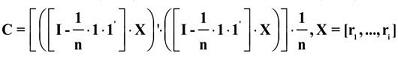

¹⁴ Assuming that these values represent the behavior of zero tracking error Exchange-Traded Funds (ETF’s) invested in each benchmark.

¹⁵ The original value of the pension fund was modified to MXN 10 000 000.00 due confidentiality issues.

¹⁷ In order to confirm that the level of volatility clustering was high in certain time periods like the aforementioned one, please refer to the historical ARCH test results shown in Appendix 2.

¹⁸ It is also when the optimization problem given in equation (3) lead to the highest concentration in the risk free asset. Refer to Chart 4 in comparison with Chart 6 to confirm this and to Appendix 2 for the probe of the presence of volatility clustering in those periods.

¹⁹ Using a T = 52 return time series length from t to t - 51.