Geostatistical modeling of clay spatial distribution in siliciclastic rock samples using the plurigaussian simulation method

Javier Méndez-Venegas*¹ and Martín A. Díaz-Viera²

¹ Instituto de Geofísica, Universidad Nacional Autónoma de México, Del. Coyoacán 04510, México D.F. *Corresponding author: lemendez84@yahoo.com.mx

²Programa de Recuperación de Yacimientos, Instituto Mexicano del Petróleo, Del. Gustavo A. Madero.

Received: March 03, 2012 ]]> Accepted: February 21, 2013
Published on line: June 28, 2013

Resumen

Con el fin de implementar esquemas de recuperación secundaria y mejorada en formaciones terrígenas complejas como los depósitos turbidíticos, el conocimiento de la distribución espacial de los granos de lutitas es un elemento crucial para la predicción del flujo de fluidos. Debido a que la interacción de los granos de lutitas con el agua puede provocar que éstas modifiquen su tamaño y/o forma, lo que causaría taponamiento de los espacios porosos y consecuentemente impacto en el flujo. En el presente trabajo, se propone una metodología para la simulación estocástica de la distribución espacial de granos obtenida a partir de imágenes de microscopio electrónico de barrido de muestras de rocas siliciclásticas. El objetivo de la metodología es obtener modelos estocásticos que permitan investigar el comportamiento de los granos de lutitas bajo diferentes condiciones de interacción físico-químicas y regímenes de flujo, y que sirvan de referencia para obtener propiedades petrofísicas (porosidad y permeabilidad) efectivas a escala de núcleo. Para la simulación estocástica espacial de los granos se utiliza el método plurigaussiano, el cual se basa en el truncado de varias funciones aleatorias Gaussianas estándar, lo cual permite manejar de manera adecuada la proporción de cada categoría y las relaciones de dependencia espacial cuando se tiene más de dos categorías o clases de grano. Los resultados muestran que los medios porosos estocásticamente simulados utilizando el método plurigaussiano reproducen adecuadamente las proporciones, las estadísticas básicas y tamaños de las estructuras de los poros presentes en las imágenes de referencia estudiadas.

Palabras clave: Geoestadística, medios porosos, monogaussiano, plurigaussiano, distribución espacial, rocas siliciclásticas.

Abstract

In order to implement secondary and enhanced oil recovery processes in complex terrigenous formations as is usual in turbidite deposits, a precise knowledge of the spatial distribution of shale grains is a crucial element for the fluid flow prediction. The reason of this is that the interaction of water with shale grains can significantly modify their size and/or shape, which in turn would cause porous space sealing with the subsequent impact in the flow. In this work, a methodology for stochastic simulations of spatial grains distributions obtained from scanning electron microscopy images of siliciclastic rock samples is proposed. The aim of the methodology is to obtain stochastic models would let us investigate the shale grain behavior under various physico-chemical interactions and flux regimes, which in turn, will help us get effective petrophysical properties (porosity and permeability) at core scale. For stochastic spatial grains simulations a plurigaussian method is applied, which is based on the truncation of several standard Gaussian random functions. This approach is very flexible, since it allows to simultaneously manage the proportions of each grain category in a very general manner and to rigorously handle their spatial dependency relationships in the case of two or more grain categories. The obtained results show that the stochastically simulated porous media using the plurigaussian method adequately reproduces the proportions, basic statistics and sizes of the pore structures present in the studied reference images.

Key words: Geostatistics, porous media, monogaussian, plurigaussian, spatial distribution, siliciclastic rock.

Introduction

The porous media characterization is a fundamental problem in areas of knowledge such as soil sciences, hydrogeology, oil reservoir, etc. Owing to the fact that the more precise knowledge one has about the porous media structure, the better the accuracy in predicting effective petrophysical properties such as porosity, permeability, capillary pressure and relative permeabilities.

In particular, in the oil industry understanding the petrophysical properties concerning the rock formation is a crucial element in reservoir management, since it allows us to accurately model the mechanisms that govern the recovery of hydrocarbons and consequently serve to propose and implement optimal secondary and enhanced recovery processes.

The aim in this work is to model the spatial grains distributions in rock samples from siliciclastic reservoir formations. As it is well known, the siliciclastic rocks are of sedimentary origin, usually formed in situ and were generated by erosion processes, transportation and deposition. Sedimentary rocks are formed by a packed grain structure that constitute the solid matrix and a pore system that is the space not occupied by the grains. The grains of the siliciclastic rocks are composed mainly of minerals such as quartz, clays, feldspars and other heavy minerals.

Usually the characterization of porous media is reduced to the study of just two categories (see section Stochastic Porous Media Reconstruction Methods), i.e. it is modeled as two phase media consisting only by rock matrix and pore space and ignoring the complex mineralogy distribution of grains that constitute the porous matrix.

Clay swelling occurs when water-base filtrates from drilling, completion, workover or simulation fluids enter the formation. Clay swelling can be caused by ion exchange or changes in water salinity. However, only clays that are directly contacted by the fluid moving in the rock will react. The nature of the reaction depends on the structure of the clays and their chemical state at the moment of contact. The most common swelling clays are smectite and smectite mixtures that create an almost impermeable barrier for fluid flow when they are located in the larger pores of a reservoir rock.

The clay swelling yields a direct impact in the reduction of pore space, and consequently in the porosity, but at the same time the spatial modification of porosity produces an alteration of the rock permeability. This is considered as a type of formation damage in which absolute rock permeability is reduced because of the alteration of clay equilibrium.

The absolute permeability is a fundamental petrophysical property of rocks and it is defined as the ability to flow or transmit fluids through a rock, conducted when a single fluid, or phase, is present in the rock. The permeability can be related with the pore space connectivity.

In this paper a novel and general methodology for stochastically reconstruction of mineralogy distribution applying the plurigaussian simulation method which far as we know it is first introduced to simulate the spatial grain distribution. In particular, the proposed methodology is applied to the clay spatial distribution in rock samples from heterogeneous siliciclastic formations to evaluate the variation of their petrophysical properties, such as porosity and permeability during a swelling process.

Stochastic porous media reconstruction methods: a brief review

The stochastic approach has been used for porous media reconstruction at pore scale in the past 20 years. The stochastic models that have been developed are basically geostatistics, which model the spatial dependency structure present in the rock structure. In particular, to represent porous media from sedimentary rock samples has been modeled the spatial distribution of grains (rock matrix) and pores (pore space). It is possible to generate a 3D model of the pore space by statistical information produced by analysis of 2D thin sections.

In their works, Adler et al. (1990) and Adler and Thovert (1998) applied the truncated Gaussian or monogaussian simulation method (Xu and Journel, 1993; Galli et al., 1994) for a porous media reconstruction from image analysis of 2D thin sections of Fontainebleau sandstone. In the truncated Gaussian method a Gaussian random function is generated and thresholded to retrieve the binary phases (pore space and rock matrix) with the correct porosity and correlation function. This method can also be extended to include more phases, such as clay.

A greater flexibility can be achieved by using the method of simulated annealing (Yeong and Torquato 1998a,b; Manwart et al. 2000; Talukdar and Torsaeter 2002; Capek et al. 2008, Politis et al. 2008). Rather than being restricted to one- and two-point correlation functions, the objective function used can be made to match additional quantities such as multi-point correlation functions, lineal-path function or pore size distribution function. Incorporating more higher-order information into the objective function, such as the local percolation probability, would most likely improve the reconstruction further, but that would also increase the computational cost of the method significantly. Although this reconstruction procedure has been more successful, the resulting images do not always capture the connectivity of pore space.

Another reconstruction methods preserving the pore size distribution, is the superposed spheres. Dos Santos et al. (2002) developed the method for reconstruct a medium upholding this statistic. The method calculates the number of spheres in order to reconstruct a given porous media, saving it is the porosity. Each sphere superposes neighboring spheres according to a user defined parameter. This method presents good results for connectivity, although it does not preserves the autocorrelation function.

Thovert et al. (2001) and Hilfer and Manswart (2001 and 2002) introduced a method that is a hybrid between the statistical and object-based methods. They verified their method using a 3D Fontainebleau sample and reported that the local percolation probability was found to be significantly better in comparison with the traditional simulated annealing. Here, local percolation probability is applied to characterize the porous media topology as a measure of connectivity (Vogel, 2002).

In their work, Casar-González and Suro-Pérez (2000, 2001 and 2003) applied the indicator simulation method and a hybrid between the multiple-point statistics and simulated annealing method. They verified their method using a carbonate rocks and reported that the results are statistically equivalent to the real porous media, i. e. both approaches reproduce correctly the histogram and the spatial variability.

Strebelle (2002) suggested a statistical algorithm in which the multiple-point statistics were inferred from exhaustive 2D training images of equivalent reservoir structures and then used to reconstruct the reservoir, adhering to any conditioning data. This method was applied successfully to both fluvial and more complex patterned reservoirs. The ability to reproduce any pattern makes this method highly attracti-ve for reconstructing complex porous media like carbonates.

In previous works about porous media reconstruction, those have been modeled as two phase media consisting only by rock matrix and pore space and ignoring the complex mineralogy distribution of grains that constitute the porous matrix. This approach possesses the disadvantage that it does not consider the mineralogical composition of the rock and consequently, these models cannot account for the chemical interaction of fluids with minerals present in the rock and even more they do not consider the dynamic alteration of petrophysical properties resulting of diagenetic processes.

In this paper we are proposing to apply the plurigaussian simulation method to simulate the spatial distribution of the mineralogical heterogeneity in the porous matrix. The choice of plurigaussian method is based on its flexibility to represent complex spatial dependencies of multiple phases. To our knowledge this method has not been applied before for this purpose. In particular, here we present the application to a case study for the distribution of clays in siliciclastic rocks. Such a model could be used to quantify the dynamic modification of the petrophysical properties of siliciclastic rocks when occur the swelling phenomenon of clays.

Data and methods

The main goals of this work are to model the geometry of the pore space by simulating grain spatial distribution from images taken in siliciclastic rock samples, as well as, the spatial distribution of clays present in the solid matrix, using spatial stochastic simulations. The procedure is applied in two successive stages. First are simulated two categories: matrix and the pore space, and subsequently is made the simulation of the mineralogy of interest.

For simulating the clay spatial distribution, we can consider two cases: the first case (case 1) is made under the assumption that clay present in the rock are allogenic, i.e., clay fragments are originally formed in other location but were transported and deposited in the pore space, therefore, clays occupy a portion of the pore space; while in the second case (case 2), clay is considered authigenic, which means that the clay was formed together with the rock and it is part of the rock matrix composition.

The images used as input data are obtained by scanning electron microscopy in backscatter electron mode. The sample preparation is similar to the one used for preparation of thin sections using light microscopy and consists of the following: the sample was impregnated with epoxy resin and polished on one side once the epoxy has hardened.

The process of extracting pores, clays and rock matrix from images of scanning electron microscopy is simpler, compared to the process for thin sections. A color thin section image contains three gray-level images in RGB space, while in scanning electron microscopy only one gray-level image is involved. In images of scanning electron microscopy, the rock matrix can be subdivided into ranges associated with different minerals using the atomic density contrast. For example, the pore space is associated with the darker gray tone because of the fact that the epoxy resin possesses smaller atomic density compared with the minerals contained in the matrix.

In the porous-media stochastic model are considered three categories: pore space, clay grains and rock matrix, where in the rock matrix category are included the rest of (no clay) mineralogies. A segmentation procedure developed by Fens (2000) enables automatic extraction of pore, clay and rock matrix categories. This procedure is based on fitting three Gaussian functions to the gray-level histogram. In images of scanning electron microscopy the gray-values represent atomic density. Prior to processing and analyzing, these gray-values have to be calibrated which takes place using a set of standards with known gray-values. This calibration is essential to make quantitative use of the data provided by the analysis. The calibration standards used here are taken from Fens (2000) and consisted of artificial reservoir rock samples that contain only quartz and epoxy.

In the case study presented, we used an image of a sandstone block obtained with the procedure described above (Figure 2), which was taken of the PhD thesis of T. Fens (Fens, 2000). The image size is 2 x 2 mm with a resolution of 256 x 256 pixels, with a pixel size equal to 0.0078 mm. In the image of Figure 2 the same five categories are clearly visible: quartz, clays, feldspars, heavy minerals and pore space. In what follows this image will be referred as the reference image.

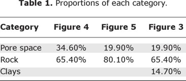
According to the objectives of this work, the reference image was initially segmented in three categories: pore space, clays and rock matrix; the last one grouped in single category: quartz, heavy minerals and feldspars (Figure 3). The resulting image has the same size as the reference image and will help us compare the simulations obtained in the latter stages of the modeling procedure. For the case 1, the reference image is segmented in two categories: black and white; where in black is represented rock matrix and in white are combined pore space and clays (Figure 4). For the case 2 is, it is applied the same procedure, but now in black are grouped rock matrix and clays while pore space is represented in white (Figure 5).

Additionally, the Euler characteristic is calculated to compare the connectivity presented in reference image versus simulations obtained. The Euler characteristic gives positive values for poorly connected structures and negative values for more connected structures (Vogel, 2002; Wu et al. 2006).

The calculation the Euler characteristic is a function of pore size (diameter), complete methodology for calculation of this characteristic is presented in Vogel (2002).

The exploratory analysis of the data is an essential phase in any practical statistical analysis. In general, it is a combination of statistical and graphical techniques that allows verifying the hypothesis that has to fulfill data sample to apply any statistical procedure. In a geostatistical analysis, it is required that the data sample fulfills the following:

a) Data sample is normally distributed or at least symmetrical.

b) Data sample must not show a significant trend; at least the intrinsic hypothesis has to be satisfied.

c) There are not distributional neither spatial outliers.

1. Basic statistics (mean, median, variance, quartiles, skewness).

2. Graphics (histogram, box plot, scatter plot, QQ plot).

Once the results of the application of these techniques are analyzed decisions can be taken to modify the data (applying transformations, excluding observations, etc.) to meet the main assumptions as far as possible or simply to take into account those assumptions that are not satisfied when the analysis is done (Armstrong and Delfiner, 1980).

The variographic or structural analysis is the most important part of the geostatistical analysis. Its aim is to model the underlying spatial structure in the data sample. In accordance to the degree of stationarity existent the data analyzed, a variogram or a covariance function can be used to determine the structure of spatial dependence. In this paper we use the variogram because it is less restrictive from the point of view of the degree of stationarity. In summary, a variographic analysis consists of the estimation of the sample variogram and to finding the variogram model that better fits it.

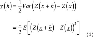
The variogram function is defined as follows:

The most common variogram estimator is given by:

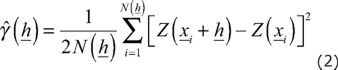
where is the number of observations pairs and and is the separation distance between them.

Geostatistical simulations consist in generating multiple realizations of a random function statistically equivalent, which means that each of the realizations has the same statistical properties that are attributed to the random function . In practice we do not know with certainty the statistical properties of the random function , therefore usually we only generate realizations that are at least statistical equivalent to the first and second-order moments present in the sample values of the random function .

Stochastic simulation method

A random function Z is a family of random variables where belongs to or some subset of it. In the one dimensional case, we prefer to speak of a stochastic process. In this work, the resulting segmented image can be viewed as a discrete or categorical random function. There are a large variety of simulation methods of categorical random functions, grouped into two families: the object models and the cells models (Chilès, 1999; Lantuejoul, 2002).

In object models each category is associated with a certain geometric shape (object) and are based on Poisson point processes, while in the cells models, a cell can take the value of one category and are based on the truncation of Gaussian random functions. Here we will use the second family of simulation methods to investigate the application.

The implementation of simulation of cells requires to characterize the discrete random function in terms of the spatial relationship of their categories, for which geostatistical analysis is done which consists of getting the proportions of occurrences of each category, the basic statistics and its variogram or the semivariance function, which is a dependence measure or spatial autocorrelation.

The proportions are calculated by dividing the sum of pixels of a given category between the total of pixels of the image, while the variogram is estimated by considering the value of the lag or interval equal to the size of the image pixel.

The proportions and the variogram obtained by categories are used as parameters in the spatial stochastic simulation method that is chosen.

Here, as a stochastic simulation method for simulating mineralogy distribution is applied the truncated plurigaussian simulation method (Galli et al., 1994; Le Loc'h and Galli, 1997; Armstrong et al., 2003). This method is a generalization of the truncated Gaussian simulation method, also known as monogaussian simulation method (Xu and Journel, 1993; Galli et al., 1994). These methods are used to simulate categorical or discrete variables, such as geological facies. The principle of these methods consists on firstly to simulate one or several standard Gaussian random functions along the study domain and afterwards they are truncated following certain spatial relationship rules in order to produce a categorical variable.

The truncated Gaussian simulation method is based only one Gaussian random function and it is summarized in Figure 6. The image (top-left) represents the standard Gaussian random function with a Gaussian model, the image (top-right) shows the histogram of a standard Gaussian distribution with two cut-offs, -0.67 and 0.12, and their respective proportion (25%, 30% and 45%). The image on the bottom, values below -0.67 are green facies, values above 0.12 are red facies and intermediate values are yellow facies. This image also shows the main limitations of the truncated Gaussian method: the anisotropy is the same for all facies and the yellow facies can touch the other two facies, but the green facies and the red facies never touch. If three or more facies were simulated in this way, they would occur in a fixed order, i.e., the method makes a hierarchy of phases when we have three or more phases.

Figure 7 illustrates the truncated plurigaussian method for the case of two Gaussian random functions and , the two Gaussian random functions used are presented at the top. The Gaussian random function on the left has its long range in the 45° while the other Gaussian random function has its long range in the 135°. The spatial relationships and contacts between units are defined by a truncation rule, this truncation rule is symbolized by a flag. The bottom (left) show the flag, which shows that there are five facies, where the facies 1,2,3,4 and facies 1,2,4,5 are in touch at the same time and the facies 3 cannot enter in contact with the facies 5. The flag also tells us the proportion of each facies in the resulting simulation. The final simulation is obtained by modeling the horizontal axis of the flag by the first Gaussian random function, while the vertical axis of the flag is modeled using the second Gaussian random function. i. e. If Z₂<Z_2B and Z₁<Z_1A, the facies is coded as green; if Z₂>Z_2B, the facies is classified as blue; if Z₂<Z_2A and Z₁<Z_1A, the facies is orange; if Z₂>Z_2A, Z₂<Z_2B and Z₁<Z_1B, the facies is coded as red and if Z₂>Z_2A, Z₂<Z_2B, Z₁>Z_1A and Z₁>Z_1B, the facies is yellow.

The truncated Gaussian method was used in the first stage, for the second stage there are three phases where all the phases considered are in contact with each other simultaneously therefore this method was discarded.

To perform the second stage, the truncated plurigaussian method was chosen because this method through the flag can control the contacts and proportions of more than two categories in a suitable way, which is the case of the present work.

Truncated plurigaussian simulation method requires the following steps:

1. Determination the thresholds at which the different standard Gaussian random function are truncated and the variogram model for each Gaussian random function.

2. Simulation of a realization of each Gaussian random function with the variogram model.

3. Application of the thresholds to the Gaussian realizations to obtain truncated plurigaussian simulation.

A detailed description of the mathematical fundaments underlying the truncated Gaussian and plurigaussian methods can be found in Armstrong et al. (2003) and Lantuejoul (2002).

Geostatical analysis

The monogaussian and plurigaussian method was applied using the reference image. During the data exploratory analysis, several statistical parameters were computed (Table 1 and Table 2); these will be used to see to what degree the simulations reproduce the statistics of the original information. This analysis concluded that the data have no outliers or trend, which was important to identify because it affects the computation of the variogram and, therefore, the model fit.

Variograms were calculated and subsequently a model was adjusted to each one of them using weighted least squares. The model with the lowest sum of squares errors was chosen and it was validated using cross validation. The leave-one-out method (Journel and Huijbregts, 1978) was used for cross-validation; which involves removing each one of the samples and estimating the value at that point using the kriging equations and the variogram model obtained. As a result, a map of the differences between actual and estimated values is obtained.

The variograms were calculated under the assumption that the information has no trend or anisotropy. These assumptions were corroborated by obtaining the variograms, because they do not have a quadratic growth and comparing the variograms in different directions, they do not show significant differences in sill, nor in range.

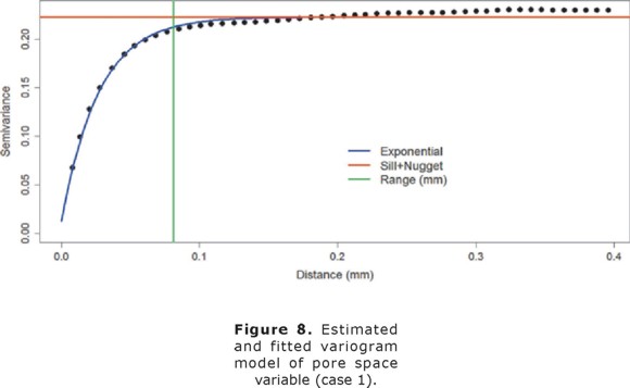
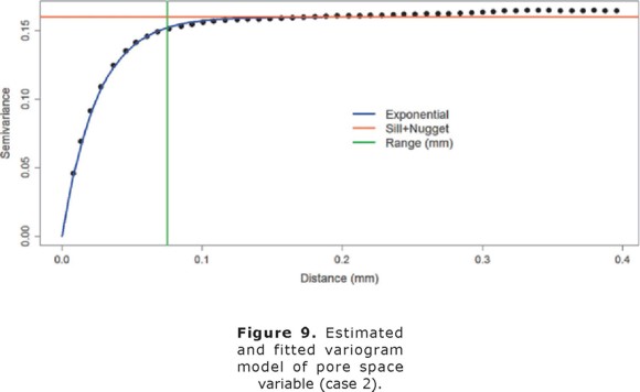
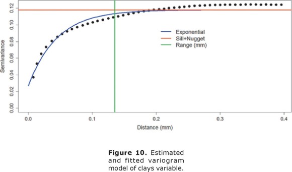
Figure 8, Figure 9 and Figure 10 show variograms for pore space (case 1 and case 2) and clays. To every variogram obtained a model was adjusted, the collection of which are presented in Table 3.

Simulation results

For simulating the first stage (case 1), we used the proportions of Figure 4 and the pore space model of Table 4. The simulation result is shown in Figure 11. Figure 11 shows on the right the flag used in the simulation. The flag only have two divisions (pore space "white" and rock "black"); the division indicates the proportion of the category in the final simulation (left).

In the second stage, consider the proportions of Figure 3. The flag used is shown in Figure 13 (right). The model used in the first Gaussian random function is the same as that used in stage 1; for the second Gaussian random function, we used the clays model (Table 3). The simulation result of this stage is shown in Figure 13.

The right of Figure 13 shows the flag, where according to the proposed case, first the pore and rock matrix is formed and then the clays, i.e. in the simulation of the first stage (Figure 11), the clays are integrated within the pore space. This is done by including another category within the category that was occupied by the pore space in the flag of the first stage. The final simulation is shown at the left of Figure 13.

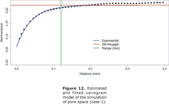
Figure 4 is the reference image of the simulation of the first stage (Figure 11). Table 4 (column 2 and 3) shows the proportions of the reference image and the simulation. The simulation adequately reproduces the image proportions, basic statistics (Table 6) and the variogram models (Table 5 and Figure 12), when models are reproduced, indicating that the simulation reproduces properly the sizes of the structures.

The result of the second stage (Figure 13) is compared with the reference image (Figure 3). Table 4 (columns 4 and 5) and Table 6 show the proportions and basic statistics of the reference image and the simulation.

Figure 15 shows the simulation of the first stage (case 2), the ingredients of the simulation with the proportions of Figure 5 and the pore space model (Table 3).

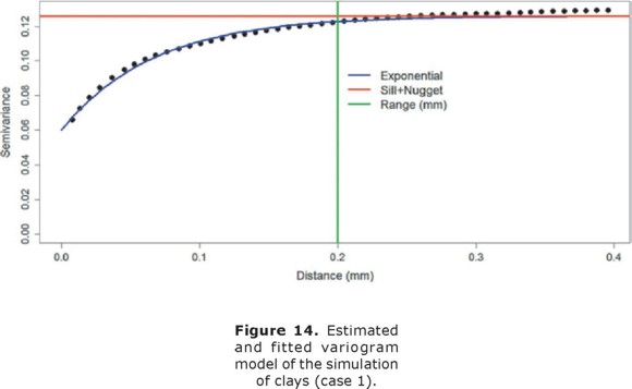
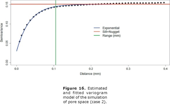
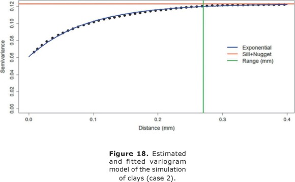
Table 7 (columns 2 and 3) and Table 8 show respectively the proportions and basic statistics of the reference image and the simulation. Variogram models for the simulation are presented in Table 9 and Figure 16 and Figure 18.

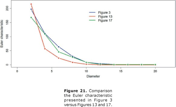
The simulation of the second stage (Figure 17) is comparable to Figure 3. Table 7 (column 4 and 5) and Table 8 present the proportions and statistics of the image and the simulation. In both phases of this case the proportions, statistics and the sizes of the structures, present in the reference images, are well reproduced.

Figure 19, Figure 20 and Figure 21 compare the Euler characteristic of the reference images with their respective simulation. The figures show the plots of the Euler characteristic versus the diameter measured in pixels of the reference images and their respective simulation (Table 10). In the three cases a very close qualitative behavior is observed. This fact could be interpreted that the simulation method reproduces quite well the connectivity behavior of reference images.

Conclusions

The results presented are preliminary. However it has been found that the simulations using the plurigaussian method adequately reproduces the proportions, basic statistics and sizes of the structures present in the studied reference images. Moreover, apparently the plurigaussian method reproduces the connectivity present in the corresponding reference image.

Although the work presented is restricted to 2D images, the methodology can be extended to 3D to achieve the reconstruction of the geometry of the porous medium, allowing a more adequate estimation of petrophysical properties.

As a future work it should be considered to combine the plurigaussian method with other methods, as might be a multipoint geostatistical simulation method (Okabe and Blunt, 2005 and 2007).

Bibliography

Adler P.M., Thovert J.F., 1998, Real porous media: Local geometry and macroscopic properties, Applied Mechanics Reviews, 51, 537-585.         [ Links ]

Adler P.M., Jacquin C.G., Quiblier J.A., 1990, Flow in simulated porous media. International Journal of Multiphase Flow, 16, 4, 691–712.         [ Links ]

Armstrong M., Delfiner P., 1980, Towards a more robust variogram: case study on coal. Fontainebleau: Springer.         [ Links ]

Armstrong M., Galli A., Le Loc'h G., Geffroy F., Eschard R., 2003, Plurigaussian Simulations in Geosciences. Springer, Berlin, 160 pp.         [ Links ]

Capek P., Hejtmánek V., Brabec L., Zikánová A., Kocirík M., 2008, Stochastic Reconstruction of Particulate Media Using Simulated Annealing: Improving Pore Connectivity, Transport in Porous Media, 76, 2, 179-198.         [ Links ]

Casar-González R., Suro-Pérez V., 2000, Stochastic imaging of vuggy formations. 2000 SPE International Petroleum Conference and Exhibition, Villahermosa, México. SPE 58998.         [ Links ]

Casar-González R., Suro-Pérez V., 2001, Two procedures for stochastic simulation of vuggy formations.. 2001 SPE Latin American and Caribbean Petroleum Conference and Exhibition, Buenos Aires, Argentina. SPE 69663.         [ Links ]

Casar-González R., 2003, Modelado estocástico de propiedades petrofísicas en yacimientos de alta porosidad secundaria. Tesis Doctoral. Facultad de Ingeniería, División de Estudios de Posgrado, Universidad Nacional Autónoma de México, Mexico.         [ Links ]

Chilès J.P., Delfiner P., 1999, Geostatistics: Modeling Spatial Uncertainty. New York:Wiley.         [ Links ]

Dos Santos L.O.E., Philippi P.C., Fernandes C.P., Gaspari H.C., 2002, Reconstrução tridimensional de microestruturas porosas com o método das esferas sobrepostas, in: Proceedings of the ENCIT 2002, Caxambu - MG, Brazil - Paper CIT02-0449.         [ Links ]

Fens T., 2000, Petrophysical Properties from Small Rock Samples Using Image Analysis Techniques. Ph.D. thesis. Netherlands: Delft University Press.         [ Links ]

Galli A., Beucher H., Le Loc'h G., Doligez B., HeresimGroup, 1994, The pros and cons of the truncated gaussian method. Geostatistical Simulations, 217-233. Dordrecht: Kluwer.         [ Links ]

Hilfer R., Manwart C., 2001, Permeability and conductivity for reconstruction models of porous media, Physical Review E., 64, 021304–021307.         [ Links ]

Lantuejoul C., 2002, Geostatistical Simulation: Models and Algorithms. Berlin: Springer.         [ Links ]

Le Loc'h G., Galli A., 1997, Truncated plurigaussian method: theoretical and practical points of view. Geostatistics Wollongong, 1, 211-222, Dordrecht: Kluwer.         [ Links ]

Manwart C., Torquato S., Hilfer R., 2000, Stochastic reconstruction of sandstones, Physical Review E., 62, 41, 365-371.         [ Links ]

Okabe H., Blunt M., 2005, Pore space reconstruction using multiple point statistics. Petroleum Science and Engineering, 46, 121-137.         [ Links ]

Okabe H., Blunt M., 2007, Pore space reconstruction of vuggy carbonates using microtomography and multiple-point statistics. Water Resources Research, 43.         [ Links ]

Politis M., Kikkinides E., Kainourgiakis M., Stubos A., 2008, Hybrid process-based and stochastic reconstruction method of porous media. Microporous and Mesoporous Materials, 110, 92-99.         [ Links ]

Strebelle S., 2002, Conditional simulation of complex geological structures using multiple-point statistics, Mathematical Geology, 34, 1-21.         [ Links ]

Talukdar M.S., Torsaeter O., 2002, Reconstruction of chalk pore networks from 2D backscatter electron micrographs using a simulated annealing technique, Journal of Petroleum Science Engineering, 33, 265–282.         [ Links ]

Thovert J.F., Yousefian F., Spanne P., Jacquin C.G., Adler P.M., 2001, Grain reconstruction of porous media: Application to a low-porosity Fontainebleau sandstone. Physical Review E., 63, 061307–061323.         [ Links ]

Vogel H.J., 2002, Topological characterization of porous media. In: Morphology and Condensed Matter - Physics and Geometry of Spatially Complex Systems. Mecke, K., and Stoyan, D. (eds.         [ Links ]), Lecture Notes in Physics, 600, 75-92.         [ Links ]

Wu K., Van Dijke M., Couples G., Jiang Z. Ma, J., Sorbie K., Crawford J., Young I., Zhang X., 2006, 3D Stochastic Modeling of Heterogeneous Porous Media – Applications to Reservoir Rocks. Transport in Porous Media 65, 443-467.         [ Links ]

Xu W., Journel A.G., 1993, GTSIM: Gaussian truncated simulations of reservoirs units in a W. Texas carbonate field. SPE 27412.         [ Links ]

Yeong C.L.Y., Torquato S., 1998a, Reconstructing random media. Physical Review E., 58, 1, 495–506.         [ Links ]

Yeong C.L.Y., Torquato S., 1998b, Reconstructing random media II Three-Dimensional from Two-Dimensional Cuts, Physical Review E., 58, 1, 224–233.         [ Links ]