Dynamic Analysis of Pneumatically Actuated Mechanisms
Arturo Lara-López, Joaquín Pérez-Meneses, José Colín-Venegas*, Eduardo Aguilera-Gómez and Jesús Cervantes-Sánchez
Mechanical Engineering Department, University of Guanajuato at Salamanca, Palo Blanco, Salamanca, Gto., México. Phone: +52 (464) 647-9940, Fax: +52 (464) 647-9940 ext. 2311 *Corresponding author email: colin@salamanca.ugto.mx
Fecha de recepción: 02-12-10 ]]> Fecha de aceptación: 22-01-10
Resumen
En este artículo se analiza el comportamiento dinámico de sistemas impulsados neumáticamente. Primeramente se analiza un modelo básico que consiste de un eslabón montado sobre un eje impulsado neumáticamente contra una fuerza externa. El modelo matemático que resulta es el fundamento básico para formular modelos de mecanismos más complejos. Luego, el análisis se extiende a un mecanismo de cuatro barras donde el eslabón de entrada se impulsa por un cilindro neumático y la fuerza externa es aplicada contra el eslabón de salida. Los modelos para ambos sistemas se obtuvieron de la aplicación directa de principios dinámicos y termodinámicos y de relaciones de la cinemática, incorporando características físicas de los mecanismos y el efecto de condiciones del aire, tamaño del tanque y amortiguamiento del pistón. Tales parámetros pueden manipularse con propósitos de diseño. Se construyeron prototipos experimentales de ambos modelos (un eslabón montado sobre un eje y un mecanismo de cuatro barras) para medir su respuesta dinámica. Los datos experimentales se compararon con la solución teórica mostrando buena similitud.
Palabras clave: Mecanismos impulsados neumáticamente, dinámica de mecanismos.
Abstract
The dynamic behavior of pneumatically driven systems is analyzed in this paper. First a basic model consisting of a single pivoted link pneumatically actuated against an external force is discussed. Resulting mathematical model is the basic foundation to formulate models for more complex mechanisms. Then, the analysis is extended to a four bar mechanism, where the input link is driven by a pneumatic cylinder and the external force is applied against the output link. Models for both systems were obtained from direct application of dynamic and thermodynamic principles and kinematics relations, incorporating physical characteristics of the mechanisms and the effect of air conditions, tank size and piston cushion. Such parameters can be manipulated for design purposes. Experimental apparatus were constructed to measure the dynamic response of both models (the single pivoted link and the four bar mechanism). Experimental data where compared with the theoretical response showing good agreement.
Key words: Pneumatically actuated mechanisms, dynamics of mechanisms.
]]> Introduction
It is a well recognized fact that increasing productivity in the high technology systems demanded by today's industry largely relies upon the ability of machines in service to run at higher speeds while still maintaining the desired dynamic behavior and precision. Many of these machines include pneumatically driven pivoted links or mechanism. Then the knowledge of the transient response of high speed linkages may be of great interest for industry to meet the compromise between speed of process and avoidance of damage to products, especially when excessive acceleration may damage products being handled. This naturally poses a challenge to machine design engineers for reliable and precise prediction of consequences resulting from an increment of the operation speed. In addition, one more difficulty is due to the inability of commercial computer-based design tools to include realistic properties in models of the dynamic behavior of pneumatic systems. Practical modeling techniques also need to be computationally efficient and should be experimentally verified, hence the motivation to write this paper.
The models presented in this article include important machine dynamic properties, such as those related to the compressed air in a tank, a pneumatic actuator with an exhaust valve that permits to regulate the start and end cushion periods and the kinematics and dynamics properties of the impulse link or mechanism, that could be under the action of external forces including dry and viscous friction and the useful force. It is expected that the contribution of this article would be centered in a new model that integrates as completely as possible the performance of the whole system, this means the pneumatic circuit with the kinematics and dynamics of the mechanism and the analysis of the influence of their parameters. In addition the resulting model is simpler than those related to similar problems previously published with no additional simplifying hypothesis. Moreover, the theoretical response of the whole system was experimentally verified.
A number of important contributions oriented to understand and predict the dynamic performance of this type of pneumatically driven devices are in the literature. A summary is presented.
Bobrow and Jabbari (1991) modeled this type of mechanism considering the rigid body equation of motion for pivoted link in addition to the energy equation for the air in the cylinder. Pressure in the inlet of the cylinder was assumed as constant. Authors emphasize the nonlinear characteristic of the system. J. Tang and G. Walker (1995) proposed a model to simulate the movement of a pneumatic actuator based on the equation of motion of a translating mass under friction force which includes dry and viscous components. That paper presents the control analysis of the system. M. Skreiner and P. Barkan (1971) proposed a model for a four bar linkage driven by a pneumatic actuator. This model was analyzed as a control system based on two equations. The first one is a kinematic equation and the second one is the control equation. Kiczkowiak (1995) proposed a model to simulate the dynamic performance of a cylinder driving links of a manufacturing machine tool. Kawakami et al (1988) proposed a model for pneumatic cylinder considering the dynamics of the piston and thermodynamics of the air. Such model shows that the heat transfer from the cylinder has little effect on movement of the piston. Authors emphasized the nonlinear characteristic of the cylinder. Aguilera and Lara (1999) proposed a model to predict the dynamic performance of a cylinder actuating on a translating mass under resistive forces taking into consideration the dimensions of the system, and basing its formulation on dynamic and thermodynamic considerations. Start and end cushion periods are considered in the modeling.
The Basic Model: a Pivoted Link.
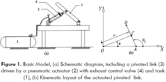
As mentioned before, the basic model includes a pivoted link driven by a pneumatic system, as shown schematically in Fig. 1. In the following subsections the analysis involved in the development of the whole theoretical model, is presented.
Joint kinematics
Figure 1 shows the schematic configuration of the actuated linkage, which can be completely described by means of the vector of joint variables q≡(r,Φ, θ2)T. These selected joint variables are related by a set of constraint equations that come from the vector loop-closure that is detected for the linkage. Similarly the joint velocity vector  and the joint acceleration vector
  are defined as function of the time derivatives of the joint variables. Thus, the vector-loop closure gives:

where L ≡ OA and p ≡ AC.
Then, given the input motion  a closed-form solution for the remaining joint variables and their time derivatives may be obtained, namely: (Shigley & Uicker, 1995)
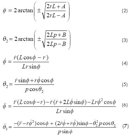
Where the involved geometric parameters (see Fig. 1) are defined as follows:
A ≡ p2- r2- L2, B ≡ p2+ L2- r2.
]]> Dynamic Analysis
Forces acting on the piston and rod are shown in Fig. 2a. It is assumed that the weight and the moment of inertia corresponding to the piston and rod are small, causing negligible normal forces NP and N0. The main reason for this assumption comes from the idea that the useful axial force on the rod F should be much greater than the weight of the cylinder.
Applying Newton's Second Law to the pivoted link (Fig. 2b and Fig. 2c), in order to find an expression for the piston force F, the resulting equations are:
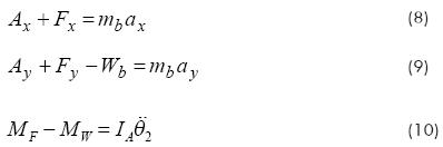
where Ax, Ay are the components of the reaction force acting on the pivoted link at point A, Fx, Fy are the components of the reaction force between piston and link, mb is the mass of the link, ax, ay are the components of the acceleration of the center of gravity of the link, MF and MW are the moments due to the useful force, F, and weight of link, Wb, about A respectively, and are given by MF≡Fpsin(Φ+θ2), Mwb≡r21Wbcosθ2, and IA is the moment of inertia of the link about point A which is defined as  for a rectangular bar (as in the experimental apparatus), with a length d.
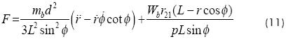
Substituting the above into equation (10) and simplifying, the following equation for the force F acting on piston is obtained:
Thermodynamic Analysis.
In order to incorporate the influence of the air properties into the whole model, the following assumptions will be considered:
]]> a) The volume of the air in the tank remains constant, b) the pressure and temperature of the air in the tank are known before expansion, c) the air behaves as an ideal gas, d) waves of pressure and temperature are neglected, e) forces against the piston include dry and viscous friction, atmospheric pressure and force on the rod, f) friction on mechanism joints is negligible, g) changes of kinetic and potential energy of the air in the system will be neglected, and h) air leakage from cylinder is negligible.The First Law of thermodynamics states that the energy entering to the control volume of a system as heat or mechanical work is transformed into a change of energy of the air contained in such control volume. For an open system and considering the space in the high pressure side of the piston as the control volume, the following equation may be written:

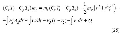
where Q is the heat transfer between the control volume and its boundary occurring during the process from an initial state (1) and any other state (2), Wair is the work done on the air contained in the control volume between the initial state 1 and a second state 2, u1 and u2 are the internal energy of air per unit of mass corresponding to states 1 and 2 respectively, h0 is the initial enthalpy of air per unit of mass, m1 and m2 are the mass of air in the control volume for initial state and a second state respectively, and min is the increment of mass in the control volume between states 1 and 2.
The principle of conservation of mass related to the control volume may be written as:

Substituting m from equation (13) into equation (12):

For ideal gases the following well known equations apply:
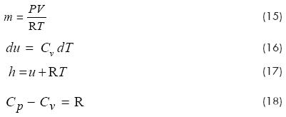
Substituting R from equation (18) into equation (17) and referring the resulting equation to the initial and a second state:
Substituting equations (19) and (20) into equation (14) it follows:
Based on the mechanical hypothesis mentioned above, the work done by the weight of piston and rod and the normal forces on these elements is not considered, being the work on the piston and rod as follows:
where Wair is the work done by the air on the high pressure side of the piston, C is the constant coefficient for viscous friction, FF is the dry friction force against the movement of the piston, F is the force on the piston rod, PA is the atmospheric pressure and AA is the piston area on the rod side.
Assuming that the process starts from the static equilibrium, then, the principle of work and kinetic energy applied to the piston and rod may be expressed as follows:
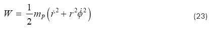
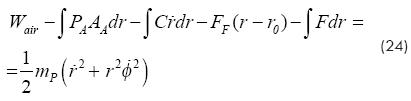
Now, substituting Wair from equation (24) into equation (21), follows that:
Now, applying Newton's Second Law to the piston (see Fig. 2a), the following equation results:
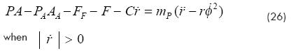
where A is the piston area on the high pressure side.
Combining equations (15) and (26) for the specific conditions of a second state, for any position of the piston, the absolute temperature for this state may be expressed as:
Where m2 is the mass of air in the control volume for such a second state, r - r0 is the displacement of the piston from the initial position to that corresponding to the second state. Substituting equations (27) and (11) into equation (25) and simplifying, the following equation may be written:
]]>
For completion of the simulation model it is necessary to use equation (29) for nozzle mass flow rate, Anderson B. W. (2001), where the factor K is given by equation (30).
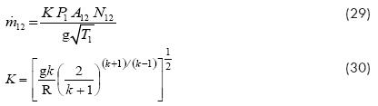
where R is the universal constant for ideal gases, g is the acceleration of gravity, A12 is the section area for flow the air, P1 and T1 are the total pressure and temperature in the state 1, that is, at the local isentropic stagnation state. The factor N12 is given by
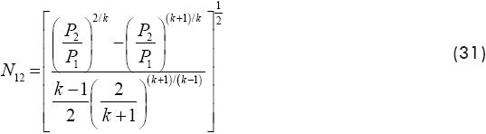
where P2 is the pressure and T2 is the temperature in the second state.
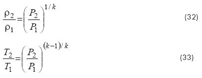
The factor N12 is a function of the ratio of specific heats and pressures. Therefore, it is nearly the same for all diatomic gases; in this case k is approximately 1.4. The isentropic process relating P1 and P2 determines the relationships between temperature and pressure and between density,p, and pressure.
These are:
]]> Simulation Procedure.
Finally, equations (6) and (28) constitute the mathematical model used to predict the dynamic performance of the system. Both equations were solved by Runge Kutta fourth order numerical method. However, those equations constitute a non linear second order system of differential equations where the variables  and
and  were both obtained itera-tively as follows; In the first iteration the initial value for the variables r and Φ, that is r0 and Φ0 were substituted into equation (28) and then using Runge Kutta numerical method that equation was solved for . The value obtained was introduced in equation (6) in order to solve for . The result from the first iteration was used as the initial value for the next iteration, and so on. The displacement of the piston is the variable that stops the iterations when its stroke is completed.
EXTENDED MODEL: FOUR BAR LINKAGE.
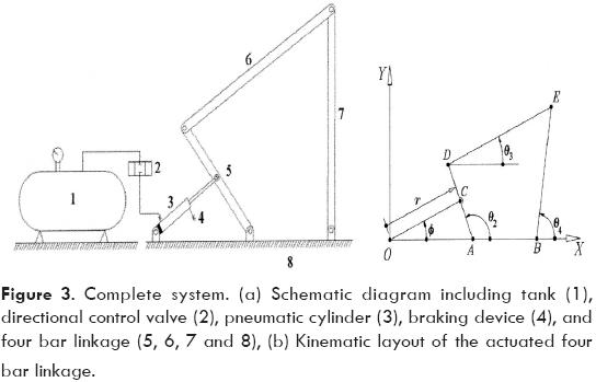
Now, the analysis made to the basic model is extended to a four bar linkage, where the input link is driven by a pneumatic system, and the external force is applied to the output link. Figure 3 shows a layout of the complete system. In the following subsections it is presented the analysis involved in the development of the whole theoretical model.
Kinematic analysis
A kinematic layout of the linkage under study is now shown in Fig. 3. In order to develop a systematic procedure, the kinematics analysis of the linkage will be divided in two parts, namely, joint kinematics and point kinematics.
]]>Joint kinematics
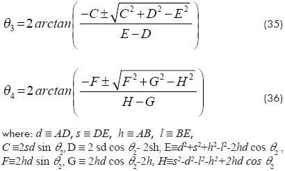
As shown in Fig. 3, the configuration of the actuated four bar linkage can be completely described by means of the vector of joint variables q≡(r,Φ,θ2,θ2, θ4)T , where r, Φ and θ2 are the joint variables defined for the basic model. The remaining joint variables θ3 and θ4 are related with θ2 by a set of constraint equations that come from the vector loop-closure that is detected for the four bar linkage. Thus, referring to Fig. 3, the vector loop-closures give the following equation in addition to equation (1):

Thus, given the input motion r a closed-form solution for the joint variables may be obtained from the following equations in addition to equations (2) and (3):
Similarly the joint velocity vector  and the joint acceleration vector
 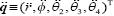 are defined as function of the time derivatives of the joint variables. Thus, given the input velocity
  and the input acceleration a closed-form solution for the remaining joint velocities and joint accelerations are defined by the following equations in addition to equations (4), (5), (6) and (7):
The solution of the acceleration equations, given by equations (6), (7), (39) and (40), completes the joint kinematics analysis.
]]> Point kinematics
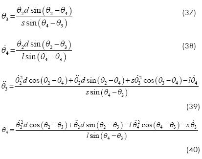
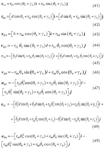
For the purposes of this paper, point kinematics means to obtain vector expressions for the position, velocity and acceleration of those linkage points which are of interest for the analyst. Moreover, they will be formulated in terms of the joint motion variables  and the geometric properties of the linkage. It is obvious that the mass center points of the moving links, G2, G3, and G4, are points of interest in the dynamic analysis. Thus, referring to Fig. 4, their corresponding position, velocity and acceleration are given by the following vectors:
being i and j unit vectors along the X and Y axis, respectively (see also Fig. 3) and the involved geometric parameters were defined as follows:
r21 ≡ AG2, r22 ≡ DG2, r32 ≡ DG3, r33 ≡ EG3, r43 ≡ EG4 and r44 ≡ BG4
Thus, expressions (47), (48), and (49) will be used presently in the equations of motion, as is shown in the next section.
]]>Dynamic analysis
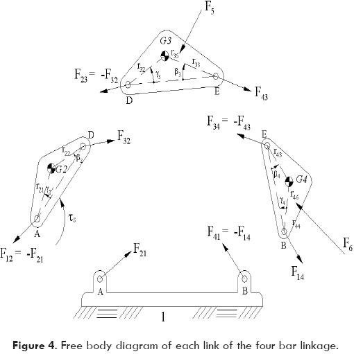
Before starting with the formulation of the equations of motion, it is necessary to make a free-body diagram for each one of the links of the four bar linkage, as it is now shown in Fig. 4. Then, according to Newton's Second Law applied for each free-body diagram, the following matrix equation may be written:
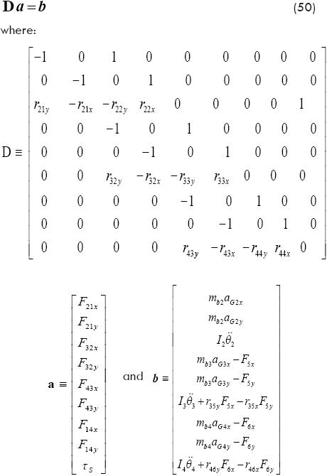
where mb2, mb3 and mb4 represent the mass of links 2, 3 and 4 respectively, and I2, I3 and I4 the mass moment of inertia of links 2, 3 and 4 respectively, and:
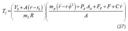
Solution of equation (50) may be found numerically or analytically. An algebraic solution was obtained by Pérez-Meneses (2003). In particular, the force on the cylinder may be obtained in terms of torque τs by the next equation, where F1 is the force applied to the linkage by the pneumatic piston:
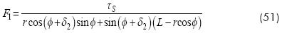
τs is the resultant torque produced by all the external forces acting on the four bar linkage. Thus, force F1 will be used into the thermodynamic equations by incorporating the work done by this force on the system.
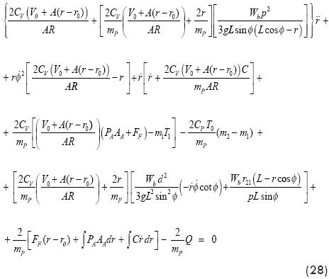
]]> Thermodynamic equations
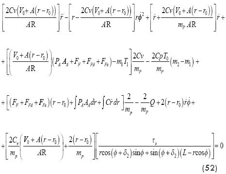
In order to incorporate the influence of the air properties into the whole model, a similar procedure to that developed for a pivoted link is follow, then applying the First Law of Thermodynamics and the basic equation for ideal gases, the following modeling equation is obtained:
In order to incorporate friction forces into the model, the following procedure is proposed:
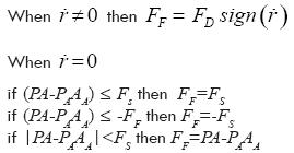
where FF is the friction force, FD is the dynamic friction force, FS is the static friction force, P is the pressure on the high-pressure side of the piston, A is the area of the inlet side of the piston, PA is the pressure on the low-pressure side of the piston, and AA is the area on the outlet side of the piston.
Simulation Procedure
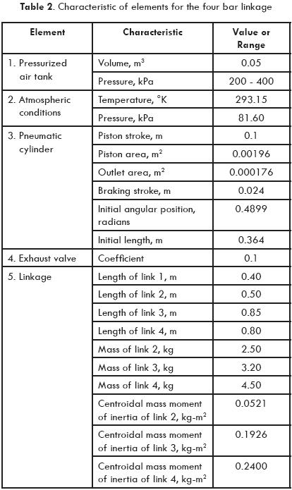
The mathematical model was run using the experimental parameters as defined in Table 2.
]]>
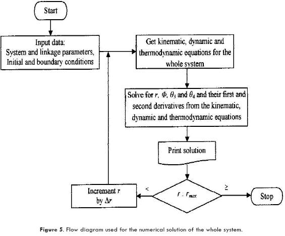
A computer program based into the flow chart presented in Fig. 5 was designed in order to solve the mathematical model. Moreover, Runge Kutta fourth order method, Korn A. G., Korn T. M. (1968), was used to integrate equations (6) and (52), using a time increment of 0.001s as the integration parameter.
EXPERIMENTAL ANALYSIS
Basic Model.
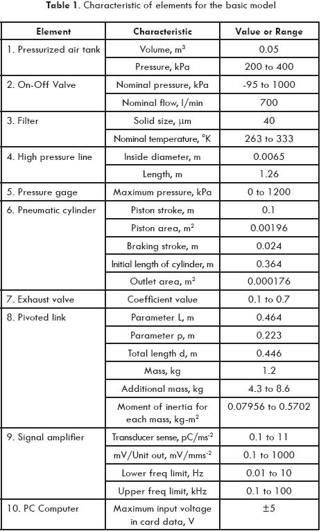
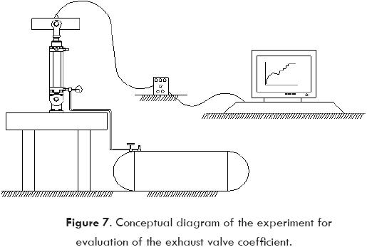
]]> The experimental apparatus used to monitor the acceleration of a point on the pivoted link is shown in Fig. 6. This includes components with characteristics as described in Table 1. Most of those characteristics were obtained from the manufacturer. The pivoted link was fabricated in the university work shop and its characteristics obtained from geometrical dimensions. A special experiment was run to adjust the coefficient value of the exhaust valve which was obtained experimentally for each one of several positions of the adjusting bolt. Fig. 7 shows the conceptual diagram of the experiment for such a purpose. The experiment was run for each position of the adjusting bolt recording the experimental response in the computer. Values of the coefficient were adjusted until the theoretical response became close to the experimental one, for a particular set of conditions. Theoretical response for this case was obtained from the following equation, Aguilera-Gomez, E. and Lara-Lopez.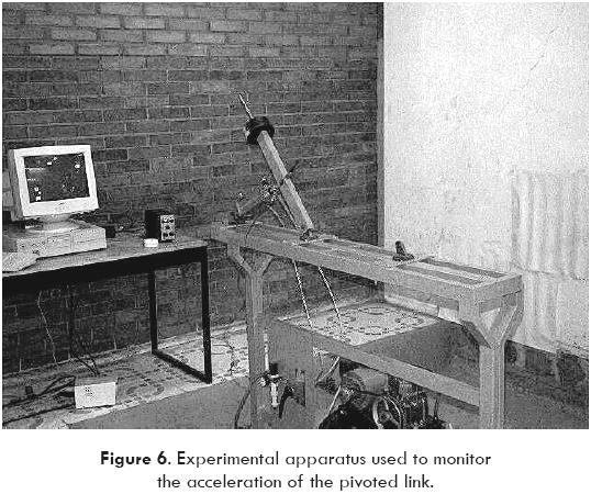
Comparison of theoretical and experimental responses
]]> Figure 8 shows the comparison of the theoretical and experimental responses, for the coefficient of exhaust valve and end cushion device. The coefficient previously determined was confirmed for several conditions varying the lifting weights and air pressure.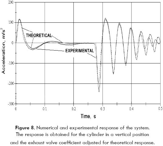
Once the values for all variables of table 1 were obtained, the mathematical model and experimental apparatus for the pivoted link were run and compared as shown in Fig. 9.
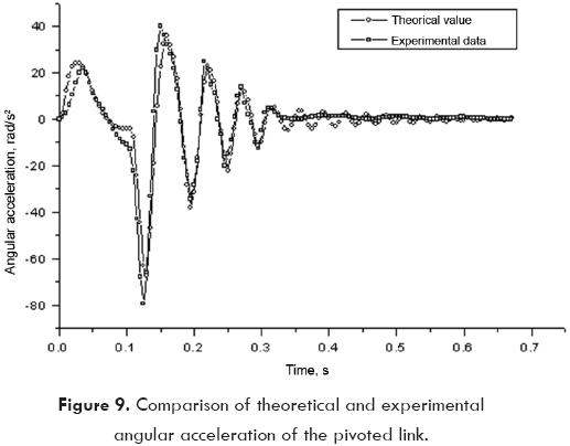
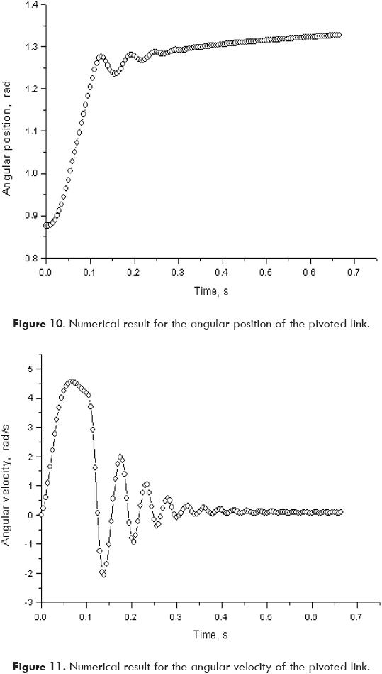
Figures 10 and 11 were obtained by numerical integration from the data corresponding to Fig. 9.
]]>
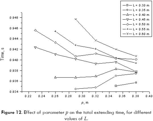
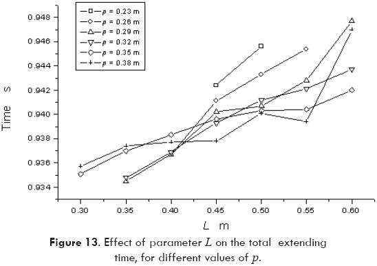
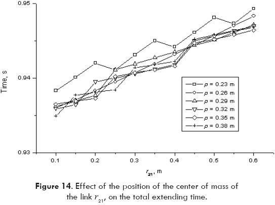
Figures 12, 13 and 14 show the effect on the response of the system due to changes on the dimensions linkage. Fig. 12 shows the effect of length of link, p, on the total extending time, maintaining the other lengths constant. Fig. 13 shows the effect of the length link L on the total extending time, and finally Fig. 14 shows the effect of the position of the link mass center r21 on the total extending time.
]]>
The difference between the theoretical response and the experimental one is about 1.5% for minimum acceleration and 3.2% for maximum acceleration. These differences may be due to an error in the transducer performance caused by changes in the temperature, calibration or humidity in the testing room.
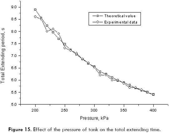
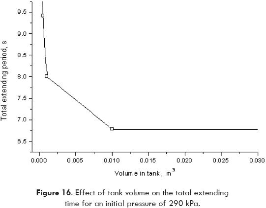
In addition, the model offers the possibility for sensitivity analysis varying a parameter of the system. An example of this feature is shown in Fig. 15 where the pressure of the tank is varied and the effect on the period of time for full extension of the cylinder can be seen. Another interesting effect can be seen in Fig. 16, where the influence of the volume of the air tank on the period for full extension is plotted for a constant initial pressure.
]]> Four bar linkage.
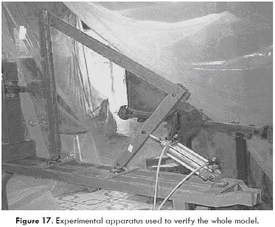
A mechanical system, similar to the one shown in Fig. 3, was designed and constructed. Such a system is shown in Fig. 17. Moreover, the external force on the output link was provided by a compression spring which is pivoted around the two extreme points. Finally, the main characteristics of the involved components are defined in Table 2.
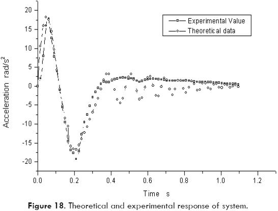
An acceleration sensor was mounted on the output link to obtain the tangential acceleration. Thus, signal from the sensor was amplified before processing the data into a PC computer Data Acquisition system. By means of computer software, plots of the acceleration as function of time were obtained. Additionally, in order to assure the confidence on the experimental results, the experiment was conducted several times. Then, the experimental response was recorded each 0.001 seconds. Figure 18 shows the response obtained in one of the experimental runs.
Comparison of theoretical and experimental responses
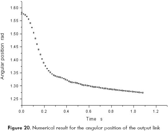
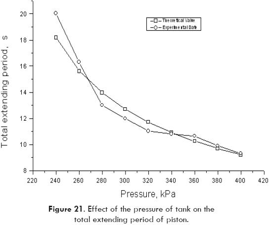
]]> Based on Fig. 18, it can be concluded that both responses, experimental and theoretical, have similar shape. However, it can be noted that the experimental response is less sensitive to oscillations probably due to dry friction on articulated joints. Moreover, the velocity and the position of the output link may be obtained by numerical integration of the theoretical response, as shown in Figs. 19 and 20. Also, the effect of any parameter of the system on the response may be predicted with the aid of the mathematical model. For instance, Fig. 21 shows the effect of tank pressure on the total extending time. Other parameters such as tank volume, air temperature, and linkage weight or linkage size may be modified in order to investigate the effect of such variables on the response of the system.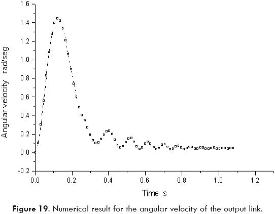
]]> CONCLUSIONS
The mathematical model based on fundamental principles of mechanics and thermodynamics allows prediction of dynamic response of the pivoted link and four bar linkages.
The shape and absolute values for the theoretical response are in good agreement with the experimental response for both cases.
Influence of system parameters may be analyzed by the proposed mathematical model, including size of components such as tank volume or dimensions of piston.
The problems discussed are highly nonlinear. However some simplifying assumptions could be made when the tank is large enough, such as considering pressure as a constant and heat exchange negligible.
The theoretical model incorporates two nonlinear ordinary differential equations. Previously published models are more complex. The incorporation of rigid body dynamic principles contributed to simplify the mathematical model.
The theoretical model may be used as a base to aid analysis, design and optimization of systems incorporating four bar linkages pneumatically driven.
Acknowledgments
Authors have a debt of gratitude with the school of Mechanical and Electrical Engineering of the University of Guanajuato at Salamanca, Mexico, for all support given to this research project. Thanks to scholarships from the National Council for Science and Technology of Mexico and from the Council for Science and Technology of the State of Guanajuato, granted to the second author, it was possible to complete the research project.
]]>REFERENCES
Aguilera-Gomez, E. and Lara-Lopez, A. Dynamics of a pneumatic system: modeling, simulation and experiments. International Journal of Robotics and Automation, 1999, 14(1), 39-43. [ Links ]
Anderson B. W. The Analysis and Design of Pneumatic Systems, 2001, Krieger publishing Company, Malabar Florida, USA. [ Links ]
Brobrow, J. E. and Jabbari, F. Adaptative pneumatic force actuation and position control. Transactions of the ASME, Journal of Dynamic Systems, Measurement and Control, 1991, 113, 267-272. [ Links ]
Kawakami, Y., Akao, J., and Kawai, S. Some considerations on the dynamic characteristics of pneumatic cylinders. Journal of Fluid Control Including Fluidics, 1988, 20, 22 - 26. [ Links ]
]]>Kiczkowiak, T. Simplified Mathematical model of the pneumatic high speed machine drive. Mechanisms and Machine Theory, 1995, 30(1), 101-107. [ Links ]
Korn A. G., Korn T. M. Mathematical Handbook for Scientists and Engineers, Second Edition,1968, McGraw-Hill Book Company, 777-785. [ Links ]
Shigley J. E. and Uicker J. J. Jr. Theory of machines and mechanisms, Second Edition, 1995, McGraw-Hill Book Company. [ Links ]
Skreiner, M. and Barkan, P. On a model of a pneumatically actuated mechanical system. Transactions of the ASME, Journal of Engineering for Industry, 1971, 93, 211-220. [ Links ]
Perez-Meneses, J. Dynamic analysis of pneumatically driven mechanisms, Doctoral Dissertation. Department of Mechanical Engineering, University of Guanajuato, 2003. [ Links ]
]]>Tang, J. and Walker, G. Variable structure control of a pneumatic actuator. Transactions of the ASME, Journal of Dynamic Systems, Measurement and Control, 1995, 117, 88-93. [ Links ]
]]>