Steam transport simulation in a geothermal pipeline network constrained by internally consistent thermodynamic properties of water

Simulación del transporte de vapor en una red geotérmica de tuberías, constreñida por propiedades termodinámicas del agua internamente consistentes

Mahendra P. Verma

Geotermia, Instituto de Investigaciones Eléctricas, Av. Reforma 113, Col. Palmira, Cuernavaca, Morelos, 62490, México. mahendra@iie.org.mx

Manuscript received: August 11, 2010
Corrected manuscript received: January 19, 2012
Manuscript accepted: September 19, 2012

ABSTRACT

A computer program, GeoSteamNet, for the numerical simulation of steam transport in geothermal pipeline networks is written in Visual Studio .NET. The program considers (a) internally consistent thermodynamic properties of water, and (b) a numerical algorithm based on the principles of conservation of mass, linear momentum (Newton's second law), and energy (the first and second laws of thermodynamics). Instability in the algorithm is observed as a consequence of ideal gas behavior of steam at low pressure, which is resolved by setting the lower limit ofpressure to 2.0×10⁵ Pa.

An ActiveX control, SteamTablesGrid, is used to calculate the thermodynamic properties of water. A study of the interrelationship among thermodynamic state variables like temperature, pressure, volume, internal energy, etc. indicates the internal consistency in the thermodynamic properties of steam only. The application of GeoSteamNet is demonstrated in the management and optimization of steam flow in a hypothetical geothermal power plant with two wells and one production unit. GeoSteamNet calculates all the parameters like fluid velocity, different types of energies such as heat loss, mechanical (kinetic and potential) energy, thermal energy, frictional energy, and total energy. Thus, the mass, linear momentum and energy balances at each nodal point in the pipeline network are used to validate the algorithm. Additionally, the computer program can also be used efficiently in the design and construction of geothermal pipeline network.

Key words: steam flow, numerical simulation, SteamTablesGrid, GeoSteamNet, PipeLine, Visual Studio .NET.

Un programa computacional, GeoSteamNet, para la simulación numérica del transporte de vapor en redes de tuberías geotermales fue escrito en Visual Studio .NET. El programa considera (a) propiedades termodinámicas del agua internamente consistentes, y (b) un algoritmo númerico basado en los principios de conservación de masa, momento lineal (segunda ley de Newton), y energía (primera y segunda leyes de la termodinámica). Se observa inestabilidad del algoritmo como consecuenca del comportamiento como gas ideal del vapor a baja presión, lo cual se resuelve configurando el límite inferior de la presión en 2.0×10⁵ Pa.

Un control ActiveX, SteamTablesGrid, en se empleó para calcular las propiedades termodinámicas del agua. Un estudio de la interrelación entre variables de estado termodinámicas como la temperatura, la presión, el volumen, la energía interna, etc. indica la consistencia interna de las propiedades termodinamicas sólo del vapor. La aplicación de GeoSteamNet se demuestra en el manejoy optimización de flujo de vapor en una planta geotérmica generadora hipotética con dos pozos y una unidad de producción. GeoSteamNet calcula todos los parámetros como velocidad del fluido, diferentes tipos de energía como pérdida de calor, energía (cinética y potencial) mecánica, energia termica, energía por fricción y energía total. De esta manera, el momento lineal y balances de energia en cada punto nodal en la red de tuberías se usan para validar el algoritmo. Adicionalmente, el programa computacional tambien puede ser usado eficientemente en el diseño y construcción de redes de tuberías geotérmicas.

Palabras clave: flujo de vapor, simulación numérica, SteamTablesGrid, GeoSteamNet, PipeLine, Visual Studio .NET.

INTRODUCTION

The steam (fluid) flow in geothermal pipeline networks is more complex than that in any other system since the pressure, temperature and flow rate of fluid in geothermal wells are controlled by nature. Additionally, the large distance among wells and their topographic settings in a geothermal field also complicate the steam flow in the pipeline networks. The well opening (i.e., controlling pressure, temperature, and flow rate at wellhead) produces incrustation problems (commonly known as silica and calcite deposits) in the geothermal reservoir as well as in the pipeline networks. Similarly, instability in the form of pressure fluctuation in the geothermal pipeline network (even sometimes in the wells) has been observed if the well openings are not synchronized. Thus, the knowledge of numerical simulation of steam flow in a pipeline network of geothermal system is vital for the rationalization and optimization of steam used in the transformation of thermal energy to electrical energy (Ruiz et al., 2010). There are two fundamental aspects to be considered for the simulation of steam transport in a geothermal pipeline network: a) internal consistency in the thermodynamic data of water, and b) appropriate algorithm. The input data for steam flow simulations are the thermodynamic properties of water; therefore, both the aspects are interrelated and the simulation results are highly influenced by the water properties.

Recent trend in the numerical simulation of complex systems is to implement ActiveX components in order to keep the integrity and transportability of huge thermodynamic databases of substances (Span, 2000). Accordingly, Verma (2003, 2009) developed the ActiveX components SteamTables and SteamTablesllE for the thermodynamic properties of water, based on the IAPWS-95 (International Association for the Properties of Water and Steam) formulation (Wagner and PruP, 2002). Lemmon et al. (2007) presented the computer program RefProp in FORTRAN for the thermodynamic and transport properties of various reference fluids, including water, although they did not mention the formulation for the water properties. However, the most accepted formulation is IAPWS-95, which is used in this work.

In the numerical simulation of systems like steam flow in a pipeline network of a geothermal system, the values of independent variables (temperature and pressure) change from point to point. The spatial grid of a geothermal pipeline network may consist of thousands of nodal points. The iteration process in the algorithm of pipeline networks stipulates the computation of the thermodynamic properties of water several times, which makes the computation very slow. Verma (2011) implemented an ActiveX control SteamTablesGrid to speed up the calculation of the thermodynamic properties of water by 200 times.

Enormous efforts have been made to understand the mechanisms of vapor transport in pipeline networks of several geothermal fields around the world (García-Gutiérrez et al., 2009). Consequently, it has resulted in the development of several computer programs: VapStat-1 (Marconcini and Neri, 1979), FLUDOF (Sánchez et al., 1987), Sims.Net (TS & E, 2005), etc. There are many recent studies on the fluid and heat flow in pipeline networks: prediction of pressure, temperature and velocity distribution of two phase flow in petroleum wells (Cazarez-Candia and Vasquez-Cruz, 2005), fluid flow characteristics with uncertainty in a geothermal well (García-Valladares et al., 2006), coupled thermo-hydraulic model for steam flow (Liu et al., 2009), a robust model for two phase fluid and heat flow in geothermal wells using the drift-flux approach (Hasan and Kabir, 2010) and others.

This article presents the development of a computer program, GeoSteamNet, for the steam transport simulation in a geothermal pipeline network, written in Visual Studio .NET. A hypothetical geothermal power plant with two wells and one production unit is analyzed to illustrate the applicability of GeoSteamNet in the management and optimization of steam transport. SteamTablesGrid is used for thermodynamic properties of water. Also, the thermo-dynamic inconsistencies in the IAPWS-95 formulation are discussed in order to illustrate the effect of thermodynamic properties of water in numerical modeling of steam transport in a geothermal pipeline network.

FUNDAMENTAL EQUATIONS

The fluid movement in a system is governed by the conservation of mass and momentum (Newton's second law or Navier-Stokes equations), and the first and second laws of thermodynamics (Smith and Van Ness, 1975; Majumdar, 1999). The second law of thermodynamics defines the direction of a spontaneous process. In the pipeline network of a geothermal power plant the steam flows from high to low pressure and heat flows from high to low temperature. Thus, the second law of thermodynamics is indirectly validated and will not be considered here. In a geothermal power plant the steam transport can be dealt quite accurately by considering certain geometrical simplification like unidirectional steady state steam flow (Verma and Arellano-G., 2010).

Continuity equation

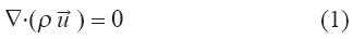
For steady state flow, the continuity equation (conservation of mass) in three dimensions is

where ρ is density and is velocity. Figure 1 shows a schematic diagram of the i^th control volume element between nodes i-1 and i. The finite difference discretization (Patankar, 1980) of continuity equation in one dimension along the pipeline is expressed as

Conservation of energy

The equation of the conservation of energy is expressed as

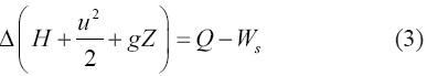
where Q is the amount of heat per unit mass given to the control volume element from surroundings; W_s is the shaft work per unit mass which is zero here; H is the enthalpy per unit mass; Z is the elevation from the reference datum line, and g is the acceleration due to gravity. Figure 1 presents a cross-sectional view of pipeline. The rate of heat transfer to the control volume element from the surroundings (Rajput, 1999) is given by

where r₁, r₂, and r₃ are radii as shown in Figure 1; k_A and k_B are the thermal conductivities of pipeline and insulation over it, respectively; h_in is the convective heat transfer coefficient between steam and inner part of the pipeline. Similarly, h_out is the convective heat transfer coefficient between outer part of insulation and surrounding air. T_inand T_out are the temperatures of inner steam and outer air, respectively.

For steady state flow, the heat transferred to the control volume element from the surroundings will be transferred to the inflowing fluid. Thus the heat added (given) to per unit mass of inflowing fluid is

The multiplying factor(1+dZ/2u) is the time required to pass the fluid through the control volume element. Thus, the discretization of energy equation is

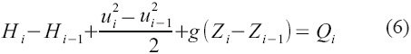
where Q_i is the amount of heat per unit mass given to i^th control volume element.

Conservation of linear momentum

The conservation of linear momentum may be written as

For both laminar and turbulent flow the energy loss due to friction is expressed with the Darcy-Weisbach equation

The Moody chart provides the value of friction coefficient f (Verma, 2008).

The discretization of momentum equation is

The conditions of pressure and temperature far from the saturation curve make the steam an ideal gas (i.e., the internal energy of steam is a function of temperature only). This creates instability in the algorithm when the pressure is lower than 5.0 × 10⁴ Pa. In the geothermal industry, steam with pressures >6.0 × 10⁵ Pa is needed to move the turbines; therefore, a parameter is implemented in the algorithm to avoid the simulation situations when pressure at any point in the pipeline network is lower than 2.0 × 10⁵ Pa.

The basic assumptions considered in the model are homogenous and unidirectional directional flow in a pipeline with the same diameter, without contractions or enlargements. Similarly, the fluid from a geothermal well is separated in a separator and the inlet fluid in the pipeline network is the saturated vapor along the liquid-vapor saturation curve. The fluid flow in a pipeline with the specified geometry is governed by three parameters: inlet pressure (or temperature), outlet pressure (or temperature), and mass flow rate. Two out of the three parameters are independent. The pipeline network is formed by the interconnection of pipelines. The steam flow calculation procedure will be described in the section, "Description of the computer program GeoSteamNet".

THERMODYNAMIC PROPERTIES OF WATER

Verma (2006) summarized the thermodynamic concepts used for understanding the relations among the state properties of a substance. Temperature (T), Pressure (P), volume (V), internal energy (U), enthalpy (H), entropy (S), Gibbs free energy (G) and Helmholtz free energy (A) including conductivity, solubility, equilibrium constant of a chemical reaction, etc. are state variables. According to thermodynamics, a pure homogeneous system is completely defined with any two independent state variables. The variation of a state function between two points is independent of the trajectory (path) and the past history of the substance (Smith and van Ness, 1975). Similarly, Verma (2006) showed that there cannot be any maximum or minimum in the behavior of a state function with an independent state variable in a pure phase when the other independent state variable is constant. In other words, a state function (or an exact function) cannot be a multi-valued function unless a phase transition exists.

P-V-T characteristics

Verma (2006) presented the T-P relationship for pure water according to the IAPWS-95 formulation. The observation made in the late 19^th century that water has a maximum density at T=277.127 K (~4°C) and P=1.0×10⁵ Pa, was called an anomalous behavior. In accordance with the laws of thermodynamics, this behavior is anomalous if the whole liquid water is considered to be a single phase. Nevertheless, recent investigations suggest the effect of hydrogen bonding on the molecular structure of water at low temperatures (see webpage of IAPWS, 2010). There are two types of structure: one associated with hydrogen bonding (below 4°C) and other without hydrogen bonding. According to the definition of "phase", a change in the structure of water molecule produces a different phase. Therefore, there is a phase transition along the minimum volume curve, and the density behavior of water is consistent in each phase according to the laws of thermodynamics.

Characteristics of U, H, S, G and A

Figure 2 shows a P-H diagram for pure water. The critical isochor curve is a separation boundary between compressed liquid and superheated steam in the fluid region. Three isotherms at T=300, 500 and 700 K are plotted. Considering T and H as independent variables, there may be two points of intersection. For example, if T=300 K and H=2.0×10⁶ J/kg, there is only one intersection (denoted by X) between the isotherm at 300 K and the H=2.0×10⁶ J/kg line within the two phase region. The water state is along the saturation curve at P=3.50×10³ Pa and the vapor fraction is 0.774. If T=500 K and H=2.0×10⁶ J/kg, there are two values: a) along the saturation curve at P=2.64x10⁶ Pa with vapor fraction of 0.561, and b) in the compressed liquid at P=1.56×10⁹ Pa. Similarly, if T=700 K and H=2.0×10⁶ J/kg, there are two values of pressure in the compressed liquid region: first at P=6.35×10⁷ and second at P=4.59×10⁸ Pa. This behavior is against the basic definition of state function. Similar behavior is observed in the characteristics of U, S, G and A (Verma, 2006).

Water properties in geothermal calculations

The future of geothermal energy is based on our understanding on the enhanced geothermal systems (MIT, 2006). The thermodynamic understanding of these systems is crucial to solving future energy demand. For example, in a deep geothermal exploration project three liquid reservoirs were found with the same characteristics except for different pressure: A) T=700 K and P=6.35×10⁷ Pa; B) T=700 K and P=1.80×10⁸ Pa; and C) T=700 K and P=4.564×10⁸ Pa. Let us analyse which geothermal reservoir will be better for electricity generation.

In the geothermal industry, the deep geothermal brine is flashed in a separator at a specified T (say 450 K) or P, and the vapor is used to move the turbines for the generation of electricity. So, the concept of mass and energy balance is expressed as

where H_R is the reservoir enthalpy (liquid), y is the fraction of vapor, and H_v and H_l are the enthalpy of liquid and vapor at the separator, respectively. Using the steam tables we can write the values of the enthalpies, and the separation of the reservoir liquid at T=450 K and P=9.30×10⁵ Pa provides values of the fraction of vapor for the three cases of (A) y=0.62, (B) y=0.56, and (C) y=0.62.

It is clear that the reservoirs A and C will produce same amount of electricity, while the reservoir B will produce slightly less electricity. So, the right answer would be the reservoir A or C. However, there should be some systematic variation in the electricity production when the reservoir pressure is changed. In these calculations all parameter have the same values, except for the reservoir liquid enthalpy. Thus, the inconsistency in the steam tables (i.e., thermo-dynamic data of water) may lead to unreliable results. The superheated steam region has internal consistent values of thermodynamic properties; however, their accuracy depends on the validation of the drastic behavior of the heat capacity, C_p near the saturation as discussed bellow.

Experimental measurements of water properties

The state functions U, H, S, G and A are mostly calculated from the PVT characteristics and heat capacity data (Verma, 2005). Therefore, to understand the thermodynamic inconsistencies in the behaviors of U, H, S, G and A, an analysis of the experimental data of C_p is presented here. Figure 3 shows the variation of experimental data of C_p with T at a specified pressure. The data were downloaded from the webpage of IAPWS (2010). The values are divided into two groups: (a) for the compressed liquid region, and (b) for the superheated steam region. The boundary is considered as the saturation curve or critical isochor.

The C_p in the compressed liquid region increases with T, and decreases with P. The variation of C_p for the whole range of P and T up to 550 K is not very significant. There is a drastic increase in the values of C_p above T=550 K, and multiple values occur just near the boundary with the vapor phase (i.e., saturation curve and critical isochor). There is a maximum near to the liquid-vapor separation boundary.

It is difficult to measure the value of C_p near to the critical point; however, according to the IAPWS formulation, the value of C_p near to critical point is very high (i.e., ~10¹² J/kg K). The critical point acts as a heat sink. In other words, there is a tremendous amount of energy in the water near the critical point. A geothermal reservoir with such conditions would be a perfect system, but it is never observed in practice.

Most of the experimental values of C_p were measured in 1956-1970 (see the database of IAPWS, 2010). The experimental details for their measurements are not clearly stated in the literature; therefore, it is difficult to state precisely the reasons for such inconsistent values. It is also amazing to note that there are no significant efforts to reproduce the experimental values of C_p since 1970.

The liquid-vapor kinetics may explain the maximum of C_p in the liquid phase region. Ground surface temperatures are quite lower than that of the water boiling point at 1.0×10⁵ Pa (1 atm). This means that the water is in the compressed liquid region, and there should not be any vapor in the atmosphere according to the thermodynamic equilibrium. Thus, the formation of atmospheric vapor is a consequence of kinetic processes.

Let consider the heating of different amounts of water in a constant volume and pressure vessel, to which pressure is applied with an inert gas. The amount of water is filled such that the pressure is higher than the saturation pressure at the corresponding T throughout the experiment. The calculations are performed with the following considerations: (i) the constant values of C_p for the liquid (4.091×10³ J/kg K) and vapor (2.787×10³ J/kg K) water corresponding to the extreme conditions of P and T, (ii) the 5% volume of vapor phase is filled with saturated vapor, and (iii) the heat of vaporization is considered as the enthalpy difference along the saturation curve. There are many limitations in these calculations; however, they successfully demonstrate the reason of the existing maximum in the behavior of C_p in the compressed liquid region.

Figure 4 presents the theoretical variation of heat capacity in two cases, (a) 0.2 kg of water at 3.0×10⁷ Pa, and (b) 0.35 kg of water at 1.0×10⁷ Pa in a reaction vessel with a volume of 0.5×10^-3 m³. The amount of water in the two cases is considered such that the whole liquid does not convert to vapor only, and that the reaction vessel does not fill completely with liquid phase in the temperature range. There is a maximum at T=629 K in the curve (a), while the curve (b) has a maximum at T=529 K. The mechanism explains successfully the existence of a maximum in the experimental data of C_p at temperatures below and near the critical point. Thus, the experimental design for the determination of liquid C_p should avoid the formation of vapor.

DESCRIPTION OF THE COMPUTER PROGRAM

GeoSteamNet

The Computer program GeoSteamNet for the numerical simulation of steam transport in geothermal pipeline networks is written in Visual Studio .NET. The thermo-dynamic data of water are calculated from the ActiveX control, SteamTablesGrid (Verma, 2011) instead of ActiveX component, SteamTables (Verma, 2003). The preliminary version of the computer program PipeCalc was written in Visual Basic 6.0 to calculate the steam flow in a pipeline (Verma and Arellano, 2010). Now, the PipeCalc is rewritten in Visual Studio .NET and is named as PipeLine. A structure variable is defined as pipe, in which all the input and calculated parameters are stored. This is done in order to create a control library when the program is tested for its functionality.

A demonstration program is written to illustrate the applicability of PipeLine. A horizontal pipeline of 1000 m is considered. All the input parameters are given in Table 1. First, a preliminary calculation was performed with varying the segment length, 1.0, 10.0 and 100.0 m. The simulation results for the segment length, 1.0 and 10.0 m were in agreement (i.e., there is no significant difference between the simulation results taking into consideration the uncertainty in the measured parameters like pressure and flow rate). Thus, the pipeline was divided into 100 elements (i.e., the length of each segment is 10.0 m) for the all simulations presented here. A small segment length increases the accuracy in the calculated values, but it also increases the execution time. So, it is always useful to perform some preliminary calculations to optimize the values of different input parameters according to the confidence limits in the measurement of these parameters. This can speed up the further calculations to obtain reliable results.

Figure 5a shows the behavior of temperature and pressure along the pipeline for three cases: i) no conduction-convection heat loss, ii) an insulation of 0.05 m thickness on the pipeline with parameters given in Table 1, and iii) maximum heat loss (i.e., no insulation). The P-T conditions in the case of no heat loss (case a) are in the superheated steam region, while the conditions of P and T are along the saturation for the cases ii and iii.

Figure 5b shows the formation of water along the pipeline during the movement of fluid. Although the steam flow is quite fast (approximately 30 m/s), a considerable amount of water is formed (about 5% by weight) at the outlet of a pipeline when there is no insulation on it.

Figure 5c shows the variation of different type of energies like heat loss, kinetic energy, thermal energy and total energy for the case iii. The fractional force converts the mechanical energy to thermal energy. Thus there is no fractional energy loss in the algorithm. The total energy at any point is the sum of the thermal energy and mechanical (kinetic and potential) energy (Figure 5c). The heat loss is the energy transferred (lost) to the environment. The sum of the total energy and heat loss at any point is the total initial energy of the system (Figure 5c). Thus, the present algorithm is validated according to the basic laws of physics.

Many empirical relations are in use in fluid mechanics, which are based on correlation studies of experimental data. For example, the coefficient of convective heat transfer is highly influenced by the local environmental conditions. So, the calibration of a numerical model for a real study system is crucial.

Steam transport in a pipeline network

To illustrate the functionality of GeoSteamNet, a hypothetical geothermal pipeline network with two wells and a power plant is considered as shown in Figure 6. The wells and the plant are interconnected with three pipelines that have the same geometrical parameters as given in Table 1. GeoSteamNet is written to solve a specific problem; however the graphic user interface of each pipeline, well and plant permits to change to values of all the parameters. Presently, a basic knowledge of programming is needed to aggregate new components in the pipeline network; however, a graphic user interface is under construction for versatility of the program. The calculation procedure used in GeoSteamNet is as follows.

Any well whose pressure is given can be considered as starting well. In the pipeline network considered here, the pressure of well 1 is given to 1,100,000 Pa (Figure 6). So, this well was considered as the starting well.

Guess value of other parameters

Either the inlet pressure or rate of steam inflow to the pipeline network is given at wellheads. If the inlet pressure is given, the rate of steam inflow is guessed and vice versa. For example, the steam inflow at well 1 is guessed to 6 kg/s. Similarly, the inlet pressure at well 2 is guessed to 1,000,000 Pa. The guess value near to the numerical solution reduces considerably the program execution time; however, user can assign any value or leave it blank.

Calculation and iteration procedure

As mentioned earlier, there are two independent variables out of inlet pressure: outlet pressure and mass flow rate in a pipeline. Thus there are three possibilities to select independent variables: (i) inlet pressure and mass flow rate, (ii) outlet pressure and mass flow rate, and (iii) inlet pressure and outlet pressure. The class PipeLine has a parameter called CalculationMethod which is assigned 1 to 3 depending of the respective situation.

In the pipeline network as shown in Figure 6 the calculation started with well 1. The outlet pressure of Pipe 1 is calculated considering the inlet pressure (given) and mass flow rate (guessed). For Pipe 2 the same outlet pressure is assigned as the calculated outlet pressure of Pipe 1. Thus the calculation is performed considering mass flow rate and outlet pressure. In Pipe 3 the outlet pressure is calculated considering inlet pressure as outlet pressure on Pipe 1, and mass flow rate as the sum of mass flow rates of Pipe 1 and Pipe 2. Now the procedure is iterated till the outlet pressure of Pipe 3 is same as that of Plant 1.

Table 2 presents the simulation results for two cases: (a) each pipeline has the parameters given in Table 1, and (b) the diameter of pipeline 3 is different (i.e., all the parameter are same as in case (a) except for the diameter of pipeline 3, which is 0.5 m instead of 0.3 m). The total mass flow rate for the scenarios 1 and 2 are 17.12 and 25.93 kg/s, respectively. The increase in the steam transport with increasing diameter of Pipe 3 validates the well known fact that the collector dimensions are very crucial in the pipeline network.

The pipeline network presented here is quite simple; however, the simulation results show various important points to be emphasized. For a specified geometry of a geothermal pipeline network there is only a certain amount of mass (vapor) that can be transported for a given wellhead pressure of all wells and power plant. The construction and modification of geothermal pipeline networks is quite costly, and the production of geothermal wells depends on nature; therefore, there is a need to perform a tolerance study of each component of the network. For example, there is a need to estimate the effect on the plant conditions of changing the pressure of well 1. The steam transport simulation computer programs are very useful for this purpose. A simulation study on the virtual pipeline network during the design of geothermal power plants can save tremendous amount of money and time (Iotovski et al., 1998).

The computer program GeoSteamNet for the numerical simulation of steam transport in geothermal pipeline networks is written in Visual Studio .NET. The algorithm is based on the conservation of mass, the linear momentum principle (Newton's second law) and the conservation of energy (i.e., first law of thermodynamics). In the pipeline network of geothermal power plant, the steam flows from high to low pressure and heat flows from high to low temperature. There is a decrease in the temperature and pressure of steam along the pipeline, even when there is no heat loss, which is associated with the expansion of steam during its flow.

The empirical relations based on correlation studies of experimental data in fluid mechanics demand the calibration of a numerical model for the real study system (e.g., the value of the coefficient of convective heat transfer) (García-Gutiérrez et al., 2009). Additionally, the algorithm presented here is constrained for the simulation of steam transport by the limitations of internal consistency in the thermodynamic properties of water. The energy balance at any point in the pipeline network validates the functionality of the present algorithm for steam transport in geothermal pipeline networks.

ACKNOWLEDGEMENTS

This work was conducted under the project "GeoSteamNet: a computer package for steam flow simulation in a pipeline network", funded by our Institute. The author appreciates the anonymous reviewers for their constructive comments which substantially improved this article.

APPENDIX A. NOMENCLATURE

A Cross-sectional area of the pipeline (m²)

C_p Heat capacity at constant pressure (J/kg K)

dF Energy loss per unit mass due to friction (J/kg)

ƒ Moody factional factor for steam flow in a pipeline

dL = (L/n) Length of control volume element (m)

g Acceleration due to gravity (m/s²)

H Enthalpy of steam (J/kg)

H_R Geothermal reservoir enthalpy (J/kg)

H_I Enthalpy of liquid phase (J/kg)

H_v Enthalpy of vapor phase (J/kg)

H_T Rate of heat transfer to the control volume element from the surroundings (J/s)

h_out Convective heat transfer coefficient between outer part of insulation and surrounding air (W/ m² K)

k_A Thermal conductivities of pipeline (W/m K)

k_B Thermal conductivities of insulation (W/m K)

L Length of pipeline (m)

 Mass flow rate of steam (kg/s)

n Number of segment in the pipeline

Q Amount of heat per unit mass given to the control volume element from surroundings (J/kg)

r₁ Inner radius of pipeline (m)

r₂ Outer radius of pipeline (m)

T_in Temperature of inner steam (K)

T_out Temperature of outer air (K)

W_s Shaft work per unit mass performed by the steam (J/kg).

 Velocity of the flowing fluid with x-component as u (m²/s)

y Fraction of vapor at the separation condition

Z Elevation of pipeline from the reference datum line at the node (m)

Subscript i Represents the value of parameter at the node or of the control volume element.

REFERENCES

Cazarez-Candia, O., Vásquez-Cruz, M.A., 2005, Prediction of pressure, temperature, and velocity distribution of two-phase flow in oil Wells: Journal of Petroleum Science and Engineering, 46, 195-208.         [ Links ]

García-Gutiérrez, A., Martínez-Estrella, J.I., Hernández-Ochoa, A.F., Verma, M.P., Mendoza-Covarrubias, A., Ruiz-Lemus, A., 2009, Development of a hydraulic model and numerical simulation of Los Azufres steam pipeline network: Geothermics, 38, 313-325.         [ Links ]

García-Valladares, O., Sánchez-Upton, P., Santoyo, E., 2006, Numerical modeling of flow processes inside geothermal wells: An approach for predicting production characteristics with uncertainties: Energy Conversion and Management, 47, 1621-1643.         [ Links ]

Hasan, A.R., Kabir, C.S., 2010, Modeling two phase fluid and heat flows in geothermal wells: Journal of Petroleum Science and Engineering, 71, 77-86.         [ Links ]

Iotovski, S., Stankov, P., Gueorguieva, D., Markov, D., 1998, A numerical procedure for pipe networks prediction, in XIX Summer School on Application of the Mathematics in Technology, Sozopol, Bulgaria: Sofia, Heron Press, 168-171.         [ Links ]

Lemmon, E.W., Huber M.L., McLinden, M.O., 2007, NIST Standard Reference Database 23: Reference Fluid Thermodynamic and Transport Properties-REFPROP, Version 8.0: Gaithersburg, National Institute of Standards and Technology, Standard Reference Data Program.         [ Links ]

Liu, Q.T, Zhang, Z.G., Pan, J.H., Guo, J.Q., 2009, A coupled thermo-hydraulic model for steam flow in pipe: Networks Journal of Hydrodynamics, Ser. B, 21, 861-866.         [ Links ]

Majumdar, A., 1999, Generalized Fluid System Simulation Program (GFSSP) Version 3.0: USA, NASA, Report No. MG-99-290, 441 pp.         [ Links ]

Marconcini, R., Neri, G., 1979, Numerical simulation of a steam pipeline network: Geothermics 7, 17-27.         [ Links ]

MIT (Massachusetts Institute of Technology), 2006, The Future of Geothermal Energy. Impact of enhanced geothermal systems (EGS) on the United States in the 21 ^st century: Massachusetts Institute of Technology, <http://www1.eere.energy.gov/geothermal/pdfs/future_geo_energy.pdf.         [ Links ]

IAPWS (International Association for the Properties of Water and Steam), 2010, A compilation of experimental data used to develop the IAPWS-95 formulation: International Association for the Properties of Water and Steam, <http://www.iapws.org>, consulted 1 October, 2009.         [ Links ]

Patankar, S.V., 1980, Numerical heat transfer and fluid flow: USA, Hemisphere Publishing Corporation, 197 pp.         [ Links ]

Rajput, R.K., 1999, Heat and mass transfer: New Delhi, India, S. Chand and Company Ltd., 691 pp.         [ Links ]

Ruiz, A., Mendoza, A., Verma, M.P., García, A., Martínez, J.I., Arellano, V, 2010, Steam flow Balance in the Los Azufres Geothermal System, Mexico: Proceedings of the World Geothermal Congress, Bali, Indonesia.         [ Links ]

Sánchez, F., Acevedo, M.A., de Santiago, M.R., 1987, Developments in geothermal energy in Mexico - Part eleven: Two-phase flow and the sizing of pipelines using the FLUDOF computer programme: Heat Recovery Systems and CHP, 7, 231-242.         [ Links ]

Smith, J. M., Van Ness, H.C., 1975, Introduction to Chemical Engineering Thermodynamics: McGraw-Hill Kogakusha, Ltd., 3^rd Ed., 632 pp.         [ Links ]

Span, R., 2000, Multiparameter equations of state: an accurate source of thermodynamic property data: Springer, Berlin, 376 pp.         [ Links ]

TS & E (Technical Software and Engineering), 2005, User's Manual for steam transmission network simulator: Richardson, TX, USA, Technical Software and Engineering, 70 pp.         [ Links ]

Verma, M.P., 2003, Steam tables for pure water as an ActiveX component in Visual Basic 6.0: Computers & Geosciences 29, 1155-1163.         [ Links ]

Verma, M.P., 2005, Procedimiento Verma para determinar propiedades termodinámica de líquidos: Boletín IIE, 29, 1-10.         [ Links ]

Verma, M.P., 2006, Thermodynamics, equations of state and experimental data-A review: Journal of Engineering and Applied Sciences, 1, 35-43.         [ Links ]

Verma, M.P., 2008, MoodyChart: an ActiveX component to calculate frication factor for fluid flow in pipelines, in Proceedings of the Thirty-Third Workshop on Geothermal Reservoir Engineering, Stanford University, Palo Alto, California.         [ Links ]

Verma, M.P., 2009, Steam Tables: An approach of multiple variable sets: Computers & Geosciences, 35, 2145-2150.         [ Links ]

Verma, M.P., 2011, SteamTablesGrid: An ActiveX control for thermo-dynamic properties of pure water: Computers & Geosciences, 37, 582-587        [ Links ]

Verma, M.P., Arellano-G., V., 2010, GeoSteamNet: 2. steam flow simulation in a pipeline, in Proceeding of the Thirty-Fifth Workshop on Geothermal Reservoir Engineering, Stanford University, Palo Alto, California.         [ Links ]

Wagner W., Pruβ A., 2002, The IAPWS formulation 1995 for the thermodynamic properties of ordinary water substance for general and scientific use: Journal of Physical and Chemical Reference Data, 31, 387-535.         [ Links ]