JENNIFER SANDRA GARCÍA-ESCALANTE, JOSÉ AGUSTÍN GARCÍA-REYNOSO, ARÓN JAZCILEVICH-DIAMANT and LUIS GERARDO RUIZ-SUÁREZ

Centro de Ciencias de la Atmósfera, Universidad Nacional Autónoma de México, Circuito de la Investigación Científica s/n, Ciudad Universitaria, 04510 México, D.F. Corresponding author: J. S. García-Escalante; e-mail: jennifer@atmosfera.unam.mx

Received July 29, 2013; accepted March 10, 2014

RESUMEN

Se utilizó un modelo de calidad del aire para analizar las emisiones provenientes de la refinería de Petróleos Mexicanos (Pemex) "Miguel Hidalgo" y la planta termoeléctrica "Francisco Pérez Ríos" de la Comisión Federal de Electricidad (CFE) localizadas en la ciudad de Tula, Hidalgo. La finalidad fue identificar la influencia de estas emisiones en la composición atmosférica de la Zona Metropolitana del Valle de México (ZMVM). El modelo utilizado acopla la meteorología y la química necesarias para la realización del estudio de impacto. Se llevó a cabo la simulación de dos escenarios que comprenden el periodo del 20 al 28 de octubre de 2008: un "escenario base" con las emisiones reales del complejo industrial y un "escenario de reducción" alternativo que supone una disminución del 40% en las emisiones de NO_x, SO₂ y compuestos orgánicos volátiles (COV) del complejo industrial. Los resultados del modelo se cotejaron con mediciones en superficie de la Red Automática de Monitoreo Atmosférico y se observó que en ciertas condiciones meteorológicas las emisiones del sector industrial sí influyen en la calidad del aire de la ZMVM. El escenario de reducción fue efectivo para simular una disminución en la concentración de SO₂ en las inmediaciones de la zona industrial e igualmente para el Valle de México; sin embargo, esta misma reducción en COV y NO_x no logró disminuir la concentración de ozono en la ZMVM.

Using an air quality model, this study shows how emissions from the "Miguel Hidalgo" refinery of Petróleos Mexicanos (Pemex) and the thermoelectric plant "Francisco Pérez Ríos" of the Comisión Federal de Electricidad (CFE, Federal Electricity Commission) in Tula, Hidalgo influence the atmosphere of the Mexico City Metropolitan Area (MCMA). The model couples meteorology and chemistry. The weather scenario encompasses the period from October 20-28, 2005. Two scenarios are compared: the first assumes a 40% reduction in emissions of NO_x, SO₂ and volatile organic compounds (VOCs) from the Tula complex (reduction scenario), and the second considers the scenario without reduction (baseline scenario). The model is compared with measurements of the Red Automática de Monitoreo Atmosférico (Automatic Environmental Monitoring Network). We observe that under certain weather conditions, the energy sector of Tula, Hidalgo affects the air quality in the MCMA. The reduction scenario is effective in reducing SO₂ concentrations; however, despite a 40% decrease in the emissions of ozone precursors, their concentrations in the MCMA did not decrease.

Keywords: Air quality modeling, Mexico City, Mexico's energy sector.

1. Introduction

The Tula industrial complex (TC) is located approximately 87 km northwest of Mexico City in the state of Hidalgo. The prevailing winds in the center of Mexico are northern during the months of September and October, so the Mexico City Metropolitan Area (MCMA), which includes Mexico City, is located downwind. Thus, 20 million inhabitants may be affected by the dispersion of emissions from this complex into the atmosphere.

The TC comprises two industrial centers: the refinery Miguel Hidalgo of Petróleos Mexicanos (Pemex), the second largest in the country, which processes approximately 279 000 barrels of oil per day (Pemex, 2013), and the thermoelectric power plant Francisco Pérez Ríos of the Comisión Federal de Electricidad (CFE, Federal Electricity Commission), which operates on a dual and combined cycle. The CFE plant is the fifth largest generation plant in the country (CEPAL-Semarnat, 2004) with an installed capacity of 1882 MW and generation of 10 210 GWh/yr. The plant uses fuel oil containing 2.6%-4% sulfur by weight, which generates high emissions of pollutants. According to the emissions inventory of 2002 for the state of Hidalgo (CEE, 2002), this thermoelectric plant emits 150 700 tons/ yr of SO₂ and 16 361 tons/yr of nitrogen oxides, while the PEMEX plant emits 173 428 tons/yr of dioxide sulfur and 16 937 tons/yr of nitrogen oxides.

Previous works by authors such as Cabrera (2008) have established TC emissions through remote sensing, while their local impact has been studied by Sosa et al. (2006) and de Foy et al. (2009). In this paper, we extend the scope of atmospheric modeling to the center of the country and incorporate photochemical phenomena, using the Multiscale Chemistry Climate Model (MCCM) (Grell et al., 2000). This model can reproduce the spatial distribution of pollutants concentrations on a complex orographic area, such as the center of Mexico, and it includes sources of anthropogenic and biogenic emissions (Jazcilevich et al., 2005). A scenario is chosen for the modeling with the required conditions for the transport of air pollutants from the TC to the Valley of Mexico. Concentration levels of SO₂ NO_x and O₃ are obtained with a spatial resolution of 3 km and a temporal resolution of 10 min in the center of Mexico. Thus, the impact of the TC emissions in the Valley of Mexico can be determined, and their effect on the air quality of this area can be determined by reducing the TC emissions in the model.

It is therefore important to establish whether the TC emissions are transported to the Valley of Mexico, and which areas and how many people are affected. With this information, the importance of the TC emissions can be measured relative to other sources that affect the atmosphere in the Valley of Mexico, and the relevance of pollution control policies for the complex can also be established.

The MCCM combines atmospheric photochemistry and meteorological modules, including gas phase chemistry, and anthropogenic and biogenic emissions, which are calculated based on data of land use, surface temperature, and radiation. The weather portion of the MCCM is based on the MM5, a fifth generation mesoscale model from the National Centers for Atmospheric Research/Pennsylvania State University (NCAR/Penn State) (Grell et al., 1994).

The MM5 includes multiple nesting capability, non-hydrostatic dynamics (Dudhia, 1993), and data assimilation in four dimensions (Strauffer and Seaman, 1994). It also simultaneously calculates meteorological and chemical changes in the domain, and generates time-dependent, three-dimensional distributions of the major organic and inorganic species relevant to the formation of oxidants such as O₃. One advantage of the online coupling of meteorology and chemistry is that it provides consistent results without data interpolation, contrasting to the uncoupled models for chemistry and transport. The system is used for prognosis and diagnosis; therefore, different modeling scenarios can be presented and their results analyzed. Finally, the output data are visualized with post-processor graphics such as GRADS (Forkel and García, 2003).

To use the MCCM anthropogenic point emission, area and linear sources are localized, and their corresponding contributions are measured. For this reason, we used databases from the Secretaría de Medio Ambiente y Recursos Naturales (Secretariat of Environment and Natural Resources) (SINE, 2003), the Gobierno del Distrito Federal (Federal District Government) (SMA-DF, 2000), and the Universidad Nacional Autónoma de México (UNAM, National Autonomous University of Mexico) (Jazcilevich et al., 2005). Information from the Red Automática de Monitoreo Atmosférico (RAMA, Automatic Environmental Monitoring Network) (SMA, 2009) is used for comparison of the meteorological and air quality variables. Effective heights from the chimneys are determined by their physical height plus the elevation that the plume reaches at the chimney outlet, according to Briggs' formulation that allows the determination of the rise of the smoke column (Wark et al., 1990).

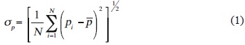
2.1 Metrics for verification of the air quality model To verify the fidelity of the model, the baseline scenario is compared with surface measurements from the using basic statistics. Standard deviations calculated from the data predicted by the model for a variable (a_p) and the observed standard deviations (cr_o) are given by Eqs. (1) and (2):

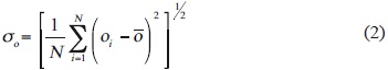
where N refers to the number of monitoring locations or points, and pi and oi are hourly average values for each monitoring station or point predicted by the model and observed, respectively.

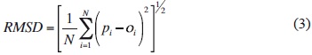
The root mean square difference (RMSD) of the mean differences between the predicted values p_i and observed o_i are also calculated with the following formula (Willmott, 1981):

With these statistical indicators, the level of accuracy of the model can be determined. The accuracy is considered high if the standard deviation of the prediction data is similar to the standard deviation of the observed data.

The RMSD (Eq. 3) is decomposed into the following:

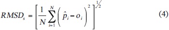
1. Systematic root mean square deviations (RMSDs) between measured and modeled values as shown in Eq. (4):

2. Unsystematic root mean square deviation (RMSDu) between measured and modeled values:

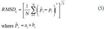
In this formula a and b are the intercept and slope, respectively, of the least squares linear regression between p and o. The RMSDs (Eq. 4) are a measure of the systematic error in the prediction model, while RMSDu (Eq. 5) describes the nonlinear discrepancy between the prediction and the observed data, which can be interpreted as a measure of accuracy.

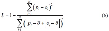
For a metric that allows verification of the model, the index of agreement I_c (Willmot et al., 1985) is defined by the following equation:

In case of the wind directions the index of similarity is used.

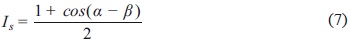
This index compares the wind directions of the prediction values with the observed values. The possible range for this index is 0 to 1. A value of 1 represents parallel vectors with same direction, 0.5 perpendicular vectors, and 0 stands for parallel vectors in opposite direction.

2.2 Nesting strategy

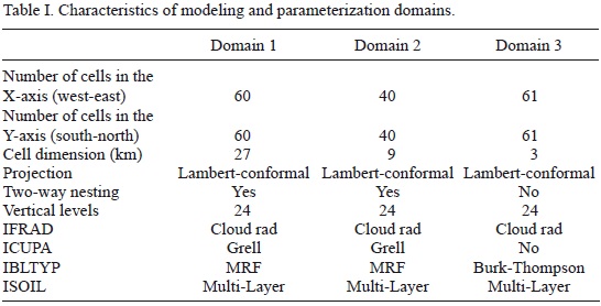
The multiple-nesting strategy employed consists of three domains that include most of Mexico and the region of influence of the TC, as shown in Figure 1. The center of the domains is located at 20.055° N, 99.278° W. Domain 1 has a resolution of 27 km, domain 2 has a resolution of 9 km, and domain 3 has a resolution of 3 km. Domain 3 covers the region of the TC and the Valley of Mexico, where the base and emission control scenarios are held.

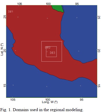
The MCCM has the ability to model the nested domains in a bidirectional manner; that is, the meteorological data between the higher and lower domains is feedbacked. Thus, bidirectional modeling is used for domains 1 and 2, but unidirectional modeling is employed for the transportation of pollutants in domain 3.

A description of the domains is shown in Table I. The three domains have 24 vertical layers. The radiation scheme (IFRAD) considers long and short waves. The cumulus parameterization is the Grell (ICUPA), used in domains 1 and 2. Turbulence schemes (IBLTYP) for the boundary layer are the medium range forecast of Hong and Pan (1996) for domains 1 and 2, and Burk and Thompson (1989) for domain 3. For the land surface temperature (ISOIL) scheme, a five-layer model is employed for moisture diffusion (Grell et al., 2000).

2.3 Scenarios, extension, severity and potential exposure

Two scenarios are proposed: base and emission control. The base scenario is the current state, and the control scenario considers a 40% reduction in emissions of SO₂, NOx, CO, and VOCs in the TC region. The control scenario is based on the fact that the refinery and thermoelectric plant can achieve those reductions by applying new technologies in a relatively short period of time. For example, the power plant could switch to a cleaner fuel such as natural gas.

To quantify the effect of the scenarios with gas criteria reductions and to make an objective comparative study, three metrics are used: extension (Ec*), severity (S), and integrated potential exposure of the population (Y) (Georgopoulos et al., 1997). The evaluation of the scenarios is performed by comparing these metrics, which are briefly described below.

Ec*: Sums the mesh elements that have exceeded the pollution standards for each gas during the episode. The formula for its calculation is as follows:

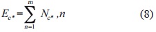
where Nc* is the number of cells in excess of concentration level c* during hour n, and m is the duration of the episode in hours.

This metric indicates the spatial extent of an episode in terms of the total number of grid cells with high pollutant values during a period.

S: Sums the times that the concentration of a criteria gas has exceeded the environmental standard. It is calculated as follows:

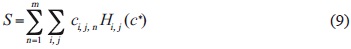
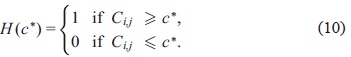
C_i,j is the concentration in the cell with coordinates and c* can be equal to the current standard level or another value of concern. The units C_i,j correspond to the same units of the gas criteria chosen for comparison.

Thus, the strategy effectiveness is a measure of the improvement of air quality in response to changes in emissions due to the controls applied. This gives a direct relation between the change in a given metric and a defined emissions reduction, and can be an indicator of the efficacy of the control strategy.

Ψ: Quantifies the extent of exposure in time and space, incorporating the size of the population potentially exposed to unhealthy levels of pollutant criteria. It is calculated using the following equation:

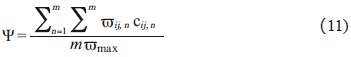
where ϖ_ijn is the population for the cell with coordinates i,j during hour n; C_jn is the concentration of cell i,j during hour n; To_max is the maximum population in the study region; and m is the number of hours in the study period (Georgopolus et al., 1997).

2.4 Modeling period and meteorological data

Meteorological data for the region of the modeling domains is obtained from the North American Regional Reanalysis (NARR) database for 2005. The data are provided every three hours with a resolution of 32 km.

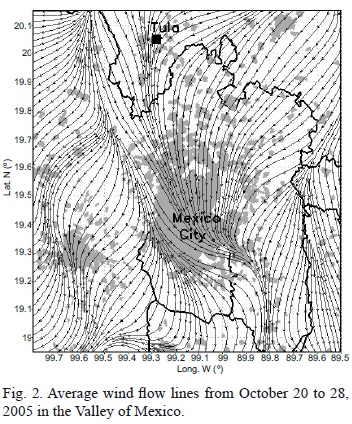
The modeling period from October 20-28, 2005 was chosen because the winds during this period come from the TC region to the Valley of Mexico. Figure 2 shows the average wind direction during October 2005. The surface flow lines demonstrate the relationship between the TC and the Valley of Mexico. This conclusion agrees with information from the Informe climatológico ambiental del Valle de México (Climatological and environmental report of the Valley of Mexico 2005) (SMA, 2006).

3. Results

Figure 3 shows an example of the time comparison of temperature, wind magnitude, and pollutant criteria concentrations that were measured and modeled at the surface at the ENEP-Acatlán (EAC) and Tlalnepantla (TLA) stations. The same comparison was also performed for the other 16 stations of the RAMA. The discontinuities indicate lack of data, and time is shown in local times.

As shown, the model acceptably describes the temperatures in the study region. Regarding SO₂ concentrations, sub- and overestimates are observed in the concentrations obtained by the model in certain periods because there are undeclared sources or the timing is unknown for the corresponding inventory.

3.1 Statistical analysis of the modeling results

We performed a basic statistical analysis described in subsection 2.1 Metrics for verification of the air quality model.

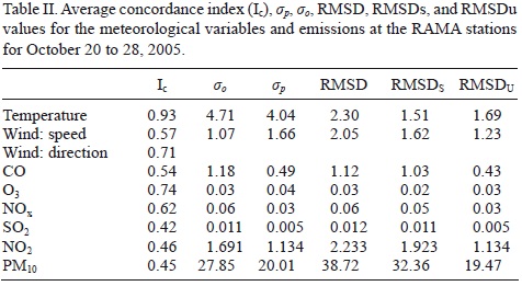
The model has an I_c concordance greater than 0.9 (where 1 is the perfect agreement) for temperature in all stations. For wind direction, the Ic ranged between 0.6 and 0.8. For wind speed, the I_c values were greater than 0.6 in the northeast stations, as shown in table II.

3.2 Spatial distribution of SO₂ concentrations by the reduction scenario

3.2.1 Sulfur dioxide (SO₂)

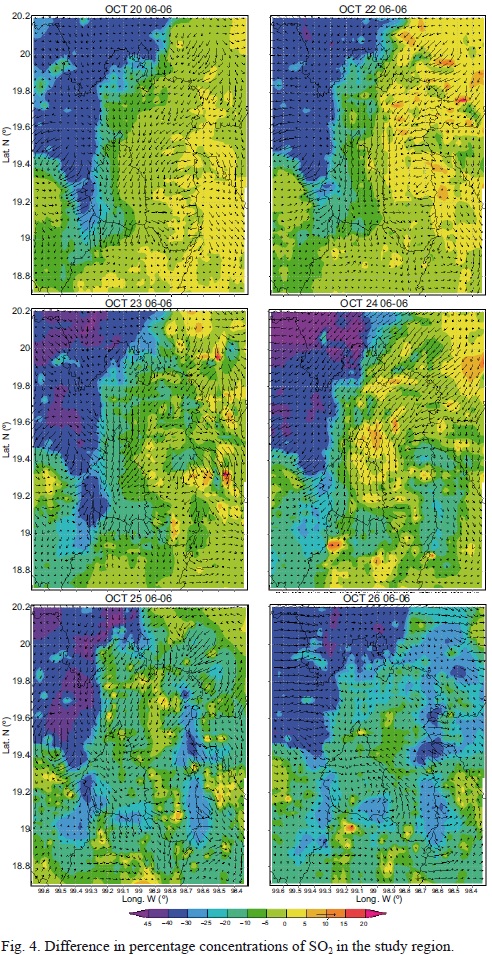
By using the MCCM model, SO₂ concentrations were obtained for both the base case scenario and the scenario for a 40% emissions reduction in the TC. The study region includes the MCMA and parts of the states of Tlaxcala, Morelos, and Hidalgo. The differences in percentages for the superficial concentrations are illustrated in Figure 4, where the maps show a 40% reduction in SO₂ emissions accounts for a decrease of 40% in concentrations around the TC and approximately 10% in the MCMA.

3.2.2 Ozone (O₃)

Maps of the percentage difference in ozone concentrations with a 40% reduction of NO_x and HC's in the TC are shown in Figure 5. There is a reduction close to the source of up to 100% of ozone, but for the rest of the region, including large areas within the MCMA, an increase of up to 10% can be observed. This increase is due to the nonlinearity of the photochemical processes.

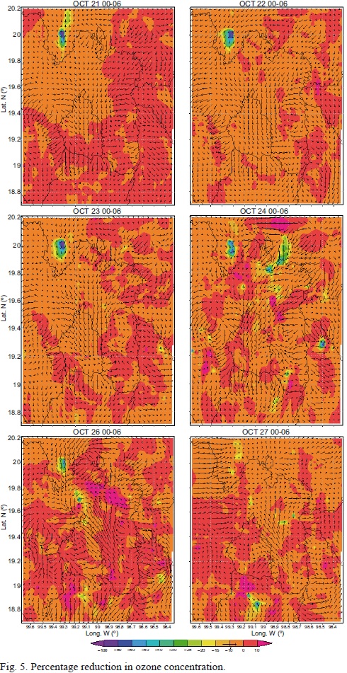
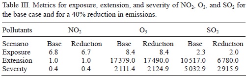
For NO₂ and O₃ there is no significant difference in the metrics for the base and the reduction scenarios. However, there is a decrease for SO₂ in the metrics of exposure, extension, and severity of 13, 35 and 42%, respectively.

4. Conclusions and discussion

Photochemical modeling shows that the TC influences the air quality in the MCMA. This mainly occurs during September and October.

With a 40% reduction in SO₂ emissions, corresponding decreases in the metrics for exposure, extension, and severity of 13, 35, and 42% are obtained in the MCMA, respectively. However, for the O3 metrics, a 40% reduction in NO₂ and HC produces a small increase in the MCMA concentrations in the emission reduction scenario compared with the baseline scenario. This result indicates that a decrease in ozone precursors in the TC does not necessarily translate to a reduction in ozone concentrations in the MCMA because of the non-linearity effects of photochemistry. Policies for pollution reduction should consider this effect. Previous works on the MCMA showed that the atmosphere is hydrocarbons-sensitive, therefore a reduction on NO_X, can induce an increment on ozone (García et al., 2009; Tie et al., 2007).

We also find that the inventory of SO₂, NO_X and maybe PM emissions needs to be improved. The MCCM underestimates these concentrations, but it was able to follow the patterns of temporal variations. There are sources of this pollutant that are not declared or are not well identified, especially in the northern part of the Valley of Mexico.

We acknowledge the Secretaría del Medio Ambiente del Distrito Federal (Secretariat of the Environment of the Federal District) for providing data from RAMA stations in the MCMA.

References

Burk S. D. and William T. Thompson, 1989. A vertically nested regional numerical weather prediction model with second-order closure physics. Mon. Wea. Rev. 111, 2305-2324.         [ Links ]

Cabrera F. C., 2008. Evaluación de un modelo de dispersión de contaminantes atmosféricos con la técnica espectroscópica DOAS pasiva. M.Sc. thesis. Centro de Ciencias de la Atmósfera, Universidad Nacional Autónoma de México, 73 pp.         [ Links ]

CEE, 2002. Inventario de emisiones del estado de Hidalgo. Consejo Estatal de Ecología. Available at: http://www.ine.gob.mx/descargas/calaire/rt3_gob_edo_hgo.pdf (last accesed on May 27, 2013).         [ Links ]

CEPAL-Semarnat, 2004. Evaluación de las externalidades ambientales de la generación termoeléctrica en México. Report. Comisión Económica para América Latina, Secretaría de Medio Ambiente y Recursos Naturales, Mexico, 59 pp.         [ Links ]

De Foy B., N. A. Krotkov, N. Bei, S. C. Herndon, L. G. Huey, A. P. Martínez, L. G. Ruiz-Suárez, E. C. Wood, M. Zavala and L. T. Molina, 2009. Hit from both sides: tracking industrial and volcanic plumes in Mexico City with surface measurements and OMI SO₂ retrievals during the MILAGRO field campaign. Atmos. Chem. Phys. 9, 9599-9617.         [ Links ]

Dudhia J., 1993. A nonhydrostatic version of the Penn State/NCAR mesoscale model: Validation tests and simulation of an Atlantic cyclone and cold front. Mon. Wea. Rev. 121, 1492-1513.         [ Links ]

Forkel R. and A. García, 2003. Manual del Multiscale Climatic Chemistry Model (MCCM). Available at: http://www.ine.gob.mx/descargas/calaire/rep_fin_proy_mccm.pdf (last accessed on May 27, 2013).         [ Links ]

García-Ruiz J., A. Jazcilevich-Diamant, L. G. Ruiz-Suárez, R. Torres-Jardón, L. M. Suárez and S. N. Reséndiz, 2009. Ozone weekend effect analysis in Mexico City. Atmósfera 22, 281-297.         [ Links ]

Georgopoulos P. G., S. Arunachalam and S. Wang, 1997. Alternative metrics for assessing the relative effectiveness of NO_x and VOC emission reductions in controlling ground-level ozone. J. Air Waste Manage. 41, 383-850.         [ Links ]

Grell G. A., J. Dudhia and D. R. Stauffer, 1994. A description of the fifth-generation Penn State/NCAR mesoscale model (MM5). NCAR Tech Note TN-398SRT. National Center for Atmospheric Research, Boulder, Colorado, 122 pp.         [ Links ]

Grell G. A., S. Emeis, W. R. Stockwell, T. Schoenemeyer, R. Forkel, J. Michalakes, R. Knoche and W. Seidl, 2000. Application of a multiscale, coupled MM5/ chemistry model to the complex terrain of the VOTALP valley campaign. Atmos. Environ. 34, 1435-1453.         [ Links ]

Hong S.-Y. and H-L. Pan, 1996. Nonlocal boundary layer vertical diffusion in a medium- range forecast model. Mon. Wea. Rev. 124, 2322-2339.         [ Links ]

Jazcilevich-Diamant A., A. García-Ruiz and E. Caetano, 2005. Locally induced surface air confluence by complex terrain and its effects on air pollution in the Valley of Mexico. Atmos. Environ. 39, 5481-5489.         [ Links ]

Molina L.T., S. Madronich, J. S. Gaffney, E. Apel, B. de Foy, J. Fast, R. Ferrare, S. Herndon, J. L. Jiménez, B. Lamb, A. R. Osornio-Vargas, P. Russel, J. J. Shauer, P. S. Stevens, R. Volkamer and M Zavala., 2010. An overview of the MILAGRO 2006 Campaign: Mexico City emissions and their transport and transformation. Atmos. Chem. Phys. 10, 8697-8760.         [ Links ]

Pemex, 2013. Segundo informe trimestral 2013. Petróleos Mexicanos, México.         [ Links ]

SINE, 2003. Inventario: fuentes fijas-1999-INEM-Hidalgo (por establecimiento). Disponible en: http://aplicaciones.semarnat.gob.mx/sine/ (last accessed May 28, 2013).         [ Links ]

SMA-DF, 2000. Inventario de Emisiones de la Zona Metropolitana del Valle de México, 1998. Secretaría de Medio Ambiente del Distrito Federal, Mexico, 225 pp. Available at: http://www.sma.df.gob.mx/sma/links/download/archivos/inventario_de_emisiones_1998.pdf (last accessed on May 27, 2013).         [ Links ]

SMA, 2006. Informe climatológico ambiental del Valle de México 2005. Secretaría de Medio Ambiente del Distrito Federal. Informe. Mexico, 198 pp. Available at: http://148.243.232.112/sma/links/download/biblioteca/flippingbooks/informe_anual_climatologico_2005/ (last accessed on May 27, 2013).         [ Links ]

SMA, 2009. Red Automática de Monitoreo Atmosférico. Secretaría de Medio Ambiente del Distrito Federal, Mexico. Available at: http://www.sedema.df.gob.mx/sedema/ (last accessed on November 17, 2009).         [ Links ]

Sosa G., C. Rivera-Cárdenas y F. Ortega-López, 2006. Medición del flujo de emisiones totales de S0₂ y NO₂ generadas por fuentes urbanas e industriales mediante detección remota. Tecnología, Ciencia, Educación 21, 103-109.         [ Links ]

Sosa G., E. Vega, E. González-Avalos, V. Mora and D. López-Veneroni, 2013. Air pollutant characterization in Tula industrial corridor, central Mexico, during the MILAGRO study. BioMed Research International 2013, art. no. 521728, http://dx.doi.org/10.1155/2013/521728.         [ Links ]

Strauffer D. R. and M. L. Seaman, 1994. Multiscale four-dimensional data assimilation. J. App.Meteorol. 33, 416-434.         [ Links ]

Tie X., S. Madronich, L. Guohui, Y. Zhuming, Z. Renyi, A. R. García, J. Lee-Taylor and L. Yubao, 2007. Characterizations of chemical oxidants in Mexico City: A regional chemical dynamical model (WRF-Chem) study. Atmos. Environ. 41, 1989-2008.         [ Links ]

Wark K. and F. C. Warner, 1990. Contaminación del aire. Origen y control. 1ª ed. Limusa, Mexico, 650 pp.         [ Links ]

Willmott C. J., 1981. On the validation of models. Phys. Geogr. 2, 184-194.         [ Links ]

Willmott C. J., S. G. Ackleson, R. E. Davis, J. J. Feddema, K. M. Klink, D. R. Legates, J. O'Donnell and M. C. Rowe, 1985. Statistics for the evaluation and comparison of models. J. Geophys. Res. 90, 8995-9005.         [ Links ]