<?xml version="1.0" encoding="ISO-8859-1"?><article xmlns:mml="http://www.w3.org/1998/Math/MathML" xmlns:xlink="http://www.w3.org/1999/xlink" xmlns:xsi="http://www.w3.org/2001/XMLSchema-instance">
<front>
<journal-meta>
<journal-id>0187-6236</journal-id>
<journal-title><![CDATA[Atmósfera]]></journal-title>
<abbrev-journal-title><![CDATA[Atmósfera]]></abbrev-journal-title>
<issn>0187-6236</issn>
<publisher>
<publisher-name><![CDATA[Universidad Nacional Autónoma de México, Instituto de Ciencias de la Atmósfera y Cambio Climático]]></publisher-name>
</publisher>
</journal-meta>
<article-meta>
<article-id>S0187-62362002000400004</article-id>
<title-group>
<article-title xml:lang="en"><![CDATA[Transfer function modeling of the monthly accumulated rainfall series over the Iberian Peninsula]]></article-title>
</title-group>
<contrib-group>
<contrib contrib-type="author">
<name>
<surname><![CDATA[MATEOS]]></surname>
<given-names><![CDATA[VIDAL L.]]></given-names>
</name>
<xref ref-type="aff" rid="A01"/>
</contrib>
<contrib contrib-type="author">
<name>
<surname><![CDATA[GARCIA]]></surname>
<given-names><![CDATA[JOSE A.]]></given-names>
</name>
<xref ref-type="aff" rid="A01"/>
</contrib>
<contrib contrib-type="author">
<name>
<surname><![CDATA[SERRANO]]></surname>
<given-names><![CDATA[ANTONIO]]></given-names>
</name>
<xref ref-type="aff" rid="A01"/>
</contrib>
<contrib contrib-type="author">
<name>
<surname><![CDATA[DE LA CRUZ GALLEGO]]></surname>
<given-names><![CDATA[MARIA]]></given-names>
</name>
<xref ref-type="aff" rid="A01"/>
</contrib>
</contrib-group>
<aff id="A01">
<institution><![CDATA[,Universidad de Extremadura Departamento de Física ]]></institution>
<addr-line><![CDATA[Badajoz ]]></addr-line>
<country>España</country>
</aff>
<pub-date pub-type="pub">
<day>00</day>
<month>00</month>
<year>2002</year>
</pub-date>
<pub-date pub-type="epub">
<day>00</day>
<month>00</month>
<year>2002</year>
</pub-date>
<volume>15</volume>
<numero>4</numero>
<fpage>237</fpage>
<lpage>256</lpage>
<copyright-statement/>
<copyright-year/>
<self-uri xlink:href="http://www.scielo.org.mx/scielo.php?script=sci_arttext&amp;pid=S0187-62362002000400004&amp;lng=en&amp;nrm=iso"></self-uri><self-uri xlink:href="http://www.scielo.org.mx/scielo.php?script=sci_abstract&amp;pid=S0187-62362002000400004&amp;lng=en&amp;nrm=iso"></self-uri><self-uri xlink:href="http://www.scielo.org.mx/scielo.php?script=sci_pdf&amp;pid=S0187-62362002000400004&amp;lng=en&amp;nrm=iso"></self-uri><abstract abstract-type="short" xml:lang="es"><p><![CDATA[Con el objeto de mejorar los resultados proporcionados por los modelos Autorregresivo - Media Móvil (ARMA) ajustados a las precipitaciones mensuales acumuladas registradas en 19 observatorios de la Península Ibérica se han usado modelos de función de transferencia (DLTFN) en los que se han empleado como variable independiente la presión local (LP), la presión a nivel del mar (SLP) o la temperatura de agua del mar (SST) en el Atlántico Norte. En todos los casos analizados, los resultados obtenidos con los modelos DLTFN, medidos mediante la varianza explicada por el modelo, han sido mejores que los resultados proporcionados por los modelos ARMA. Los mejores resultados han sido dados por aquellos modelos que usan la presión local como variable de entrada, seguidos por los modelos que emplean la presión a nivel del mar, siendo los modelos que emplean la temperatura del agua del mar los que peores resultados proporcionan. Con referencia a la situación geográfica, los modelos ajustados a los observatorios localizados al oeste de la Península dan mejores resultados que los ajustados a los observatorios situados al norte y este de la misma. Asimismo se ha encontrado que existe una región en el Atlántico Norte situada entre los paralelos 0º y 20°N donde la temperatura del agua parece tener alguna influencia sobre las precipitaciones peninsulares. Esta región se traslada hacia el norte cuando se emplean presiones a nivel del mar, a la vez que se intensifica su influencia.]]></p></abstract>
<abstract abstract-type="short" xml:lang="en"><p><![CDATA[In order to improve the results given by Autoregressive Moving-Average (ARMA) modeling for the monthly accumulated rainfall series taken at 19 observatories of the Iberian Peninsula, a Discrete Linear Transfer Function Noise (DLTFN) model was applied taking the local pressure series (LP), North Atlantic sea level pressure series (SLP)and North Atlantic sea surface temperature (SST) as input variables, and the rainfall series as the output series. In all cases, the performance of the DLTFN models, measured by the explained variance of the rainfall series, is better than the performance given by the ARMA modeling. The best performance is given by the models which take the local pressure as the input variable, followed by the sea level pressure models and the sea surface temperature models. Geographically speaking, the models fitted to those observatories located in the west of the Iberian Peninsula work better than those on the north and east of the Peninsula. Also, it was found that there is a region located between 0°N and 20°N, which shows the highest cross-correlation between SST and the peninsula rainfalls. This region moves to the west and northwest off the Peninsula when the SLP series are used.]]></p></abstract>
<kwd-group>
<kwd lng="en"><![CDATA[Autoregressive - Moving Average]]></kwd>
<kwd lng="en"><![CDATA[Discrete Linear Transfer Function Noise]]></kwd>
<kwd lng="en"><![CDATA[Rainfall Modeling]]></kwd>
</kwd-group>
</article-meta>
</front><body><![CDATA[  	    <p align="center"><font face="verdana" size="4"><b>Transfer function modeling of the monthly accumulated rainfall series over the Iberian Peninsula</b></font></p>  	    <p>&nbsp;</p>  	    <p align="center"><font face="verdana" size="2"><b>VIDAL L. MATEOS, JOSE A. GARCIA, ANTONIO SERRANO and MARIA DE LA CRUZ GALLEGO</b></font></p>  	    <p align="center"><font face="verdana" size="2"><i>Dpto. de F&iacute;sica, Universidad de Extremadura, 06071 Badajoz, Spain</i></font></p>  	    <p>&nbsp;</p>  	    <p align="center"><font face="verdana" size="2">(Manuscript received June 12, 2001; accepted in final form April 3, 2002)</font></p>  	    <p>&nbsp;</p>  	    <p align="justify"><font face="verdana" size="2"><b>RESUMEN</b></font></p>  	    <p align="justify"><font face="verdana" size="2">Con el objeto de mejorar los resultados proporcionados por los modelos Autorregresivo &#45; Media M&oacute;vil (ARMA) ajustados a las precipitaciones mensuales acumuladas registradas en 19 observatorios de la Pen&iacute;nsula Ib&eacute;rica se han usado modelos de funci&oacute;n de transferencia (DLTFN) en los que se han empleado como variable independiente la presi&oacute;n local (LP), la presi&oacute;n a nivel del mar (SLP) o la temperatura de agua del mar (SST) en el Atl&aacute;ntico Norte.</font></p>  	    ]]></body>
<body><![CDATA[<p align="justify"><font face="verdana" size="2">En todos los casos analizados, los resultados obtenidos con los modelos DLTFN, medidos mediante la varianza explicada por el modelo, han sido mejores que los resultados proporcionados por los modelos ARMA. Los mejores resultados han sido dados por aquellos modelos que usan la presi&oacute;n local como variable de entrada, seguidos por los modelos que emplean la presi&oacute;n a nivel del mar, siendo los modelos que emplean la temperatura del agua del mar los que peores resultados proporcionan.</font></p>  	    <p align="justify"><font face="verdana" size="2">Con referencia a la situaci&oacute;n geogr&aacute;fica, los modelos ajustados a los observatorios localizados al oeste de la Pen&iacute;nsula dan mejores resultados que los ajustados a los observatorios situados al norte y este de la misma. Asimismo se ha encontrado que existe una regi&oacute;n en el Atl&aacute;ntico Norte situada entre los paralelos 0<sup>o</sup> y 20&deg;N donde la temperatura del agua parece tener alguna influencia sobre las precipitaciones peninsulares. Esta regi&oacute;n se traslada hacia el norte cuando se emplean presiones a nivel del mar, a la vez que se intensifica su influencia.</font></p>  	    <p>&nbsp;</p>  	    <p align="justify"><font face="verdana" size="2"><b>ABSTRACT</b></font></p>  	    <p align="justify"><font face="verdana" size="2">In order to improve the results given by Autoregressive Moving&#45;Average (ARMA) modeling for the monthly accumulated rainfall series taken at 19 observatories of the Iberian Peninsula, a Discrete Linear Transfer Function Noise (DLTFN) model was applied taking the local pressure series (LP), North Atlantic sea level pressure series (SLP)and North Atlantic sea surface temperature (SST) as input variables, and the rainfall series as the output series. In all cases, the performance of the DLTFN models, measured by the explained variance of the rainfall series, is better than the performance given by the ARMA modeling. The best performance is given by the models which take the local pressure as the input variable, followed by the sea level pressure models and the sea surface temperature models. Geographically speaking, the models fitted to those observatories located in the west of the Iberian Peninsula work better than those on the north and east of the Peninsula. Also, it was found that there is a region located between 0&deg;N and 20&deg;N, which shows the highest cross&#45;correlation between SST and the peninsula rainfalls. This region moves to the west and northwest off the Peninsula when the SLP series are used.</font></p>  	    <p align="justify"><font face="verdana" size="2"><b>Keywords:</b> Autoregressive &#45; Moving Average, Discrete Linear Transfer Function Noise, Rainfall Modeling.</font></p>  	    <p>&nbsp;</p>  	    <p align="justify"><font face="verdana" size="2"><b>1.&nbsp;Introduction</b></font></p>  	    <p align="justify"><font face="verdana" size="2">Autoregressive Moving Average (ARMA) models have frequently been used to parameterize accumulated monthly rainfall series (Delleur and Kavvas, 1978; Katz and Skaggs, 1981) and specifically to the Iberian Peninsula by Garrido and Garc&iacute;a (1993). In these models the rainfall series is regressed over itself lagged behind in time plus random noise. In an attempt to improve the results given by the ARMA models, Discrete Linear Transfer Function Noise models (DLTFN) were used (Box and Jenkins, 1976). There supposedly is a dynamic system where some variables (the predictors) act as inputs of this kind of model's system, and others (the predictands) as outputs, and that a change in the level of the input variables will produce a change in the output variables, though not necessarily at the same time. This implies a causal relation, in a statistical sense, between the input and output of the system. In the present paper the accumulated monthly rainfall series is taken as the output variable. For the input variables, one of the following is selected: monthly mean sea surface temperature (SST), which could be taken as a measure of the exchange of Sensible and Latent Heat between the ocean and the atmosphere, monthly mean sea level pressure (SLP), and monthly mean local station surface pressure (LP) (pressure measured at the same location as the accumulated monthly rainfall). The election of these variables was determined by the fact that according to Lin&eacute;s (1981) a good deal of the rainfall over the Iberian Peninsula is due to frontal systems coming from the North Atlantic Ocean, so that one might expect that a relation between the rainfall series measured over the Iberian Peninsula and the SST and SLP series over the North Atlantic Ocean could be established. The existence of such teleconnections between SST and SLP over the North Atlantic Ocean and large scale weather over Europe has been demonstrated by, amongst others, Ratcliffe and Murray (1970), Meehl and van Loon (1979), Barnett (1984). More specifically, the relation between SST and rainfall series has been studied, for example, by Nicholls (1989) in Australia, by Hastenrath <i>et al.</i> (1995) in South Africa, and in the Sahel by Folland <i>et al.</i> (1986), and Fontaine <i>et al.</i> (1995).</font></p>  	    <p>&nbsp;</p>  	    ]]></body>
<body><![CDATA[<p align="justify"><font face="verdana" size="2"><b>2.&nbsp;Data</b></font></p>  	    <p align="justify"><font face="verdana" size="2">The data to be analyzed in this study can be divided into two groups:</font></p>  	    <p align="justify"><font face="verdana" size="2"><i>a. Continental data</i></font></p>  	    <p align="justify"><font face="verdana" size="2">
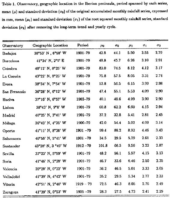
These data account for the accumulated monthly rainfall series measured at 19 observatories throughout the Iberian Peninsula, whose geographic situation is given in <a href="#t1">Table I</a> and displayed in <a href="#f1">Figure 1</a>. It also indicates the mean monthly pressure series measured at those observatories. This set of observatories coincides practically with that used by Lorente (1985) and Lin&eacute;s (1981), and could be considered representative of the Iberian Peninsula. Most of the temporal series extend from 1901 to 1979.</font></p>  	    <p align="center"><font face="verdana" size="2"><a name="t1"></a></font></p>  	    <p align="center"><font face="verdana" size="2"><img src="/img/revistas/atm/v15n4/a4t1.jpg"></font></p>  	    <p align="center"><font face="verdana" size="2"><a name="f1"></a></font></p>  	    <p align="center"><font face="verdana" size="2"><img src="/img/revistas/atm/v15n4/a4f1.jpg"></font></p>  	    <p><font face="verdana" size="2"><i>b. Ocean data</i></font></p>     <p align="justify"><font face="verdana" size="2">
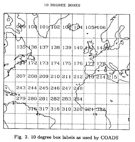
These data correspond to SST and SLP, and were obtained from groups 3 and 4 of the COADS (Comprehensive Ocean&#45;Atmosphere Data Set) produced by the National Climatic Data Center of the USA (Woodruff <i>et al.,</i> 1987). Both groups average over 10 degree latitude&#45;longitude boxes in the region 0&deg; N to 70&deg; N and 10&deg; E to 70&deg; W. <a href="#f2">Figure 2</a> shows the box labels as used by COADS. The period spanned by these series also run from 1901 to 1979. The SST and SLP series were selected for subsequent analysis for each observatory in the Peninsula. These series, once deseasonalized and linear detrended, have the highest cross&#45;correlation coefficient with each rainfall series square root transformed, deseasonalized and linear detrended (see below).</font></p>  	    ]]></body>
<body><![CDATA[<p align="center"><font face="verdana" size="2"><a name="f2"></a></font></p>  	    <p align="center"><font face="verdana" size="2"><img src="/img/revistas/atm/v15n4/a4f2.jpg"></font></p>  	    <p align="justify"><font face="verdana" size="2"><a href="#t2">Tables 2</a> and <a href="#t3">3</a> present the highest correlation coefficient of each rainfall series with the SST and SLP series respectively, along with their standard errors, estimated as &plusmn;1.96 times the lag&#45;zero cross&#45;correlation coefficient variance, which is given by Bennett (1979).</font></p>  	    <p align="center"><font face="verdana" size="2"><a name="t2"></a></font></p>  	    <p align="center"><font face="verdana" size="2"><img src="/img/revistas/atm/v15n4/a4t2.jpg"></font></p>  	    <p align="center"><font face="verdana" size="2"><a name="t3"></a></font></p>  	    <p align="center"><font face="verdana" size="2"><img src="/img/revistas/atm/v15n4/a4t3.jpg"></font></p>  	    <p align="center"><font face="verdana" size="2"><img src="/img/revistas/atm/v15n4/a4e0.jpg"></font></p>  	    <p align="justify"><font face="verdana" size="2">where <i>r<sub>xx</sub></i> is the autocorrelation coefficient at lag <i>k</i> for the input series (SLP or SST), <i>r<sub>yy</sub></i> is the autocorrelation coefficient at lag <i>k</i> for the output series (rainfall series) and <i>r<sub>xy</sub></i> is the cross&#45;correlation coefficient at lag <i>k</i> between the input and the output series. <i>T</i> is the period spanned by the series. The above sum was truncated at <i>T</i>/<i>4.</i></font></p>  	    <p align="justify"><font face="verdana" size="2">The labels of the boxes with which the highest cross&#45;correlation value is obtained and the significance level, the probability that the cross&#45;correlation coefficient is significantly different from zero, determined using a bootstrap procedure (Efrom, 1993; Kahl <i>et al.,</i> 1993) are also indicated. As observed in the SST table, except for Barcelona, Santander, Vitoria and Salamanca, the most repeated box is # 248 (see <a href="#f2">Figure 2</a> for the location of the boxes). To further analyze the relationship between the SST series and the rainfall series, a contour plot of the cross&#45;correlation between each rainfall series and all the SST series was made. <a href="/img/revistas/atm/v15n4/a4f3.jpg" target="_blank">Figure 3</a> shows four cases (Evora, Madrid, Santander and Valencia) out of the nineteen contour plots obtained. As suggested by the Evora and Madrid plots, there is a belt from 20&deg; N to 30&deg; N and 10&deg; W to 70&deg;W that presents, however, significant positive cross&#45;correlations between the SST and the the rainfall series. The results obtained for these two observatories are typical examples of those located in the west and southwest of the Peninsula. This is more clearly seen in <a href="#f2">Figure 2</a>, which is a contour&#45;plot of the cross&#45;correlations between box # 248 and all of the rainfall series. Also, it was found that for some observatories (Coimbra, Evora, S. Fernando, Lisboa, Malaga, Oporto, Sevilla and Soria) there is a small area north of the positive cross&#45;correlation region, with significant negative cross&#45;correlation, leading to a kind of dipole with the positive cross&#45;correlation region. An analysis of the cross&#45;correlations between the rainfall series and the SST series formed as the difference between the positive and the negative region do not seem to improve the results obtained with the SST themselves. Hence, the SST series of the box with the maximum cross&#45;correlations with the rainfall series will be used in subsequente analysis. As shown by Rowntree (1976), using a hemispheric model, a tropical ocean temperature anomaly causes a fall in surface pressure which extends well north of 60&deg;N, which in turn induces an increase in rainfall at middle latitudes. These theoretical results match with our finding of a relationship between box # 248 and the rainfall over the Iberian Peninsula.</font></p> 	    ]]></body>
<body><![CDATA[<p align="center"><img src="/img/revistas/atm/v15n4/a4f4.jpg"></p>      <p align="justify"><font face="verdana" size="2">With reference to the SLP table, except for Barcelona, Santander, Vitoria and Zaragoza, boxes with greater cross&#45;correlations are adjacent to the north, west and southwest of the Iberian Peninsula (boxes # 176, 177 and 212). In this case, the cross&#45;correlation coefficients are notably higher than those obtained for the SST series, and they are negative, which means that the highest precipitations are obtained with low pressure centers situated in or near these boxes. As before, we made contour plots of the cross&#45;correlation between each rainfall series and the SLP series, <a href="/img/revistas/atm/v15n4/a4f5.jpg" target="_blank">Figure 5</a> shows four examples of the contour plots obtained. The results for Evora and Madrid are representative of those obtained at observatories located in western and southwestern Spain. As the figure shows, the region in boxes # 176 and 212 presents the highest (negative) cross&#45;correlation values. The relation between the rainfall over the Peninsula and the SLP over the above mentioned boxes is more clearly seen in <a href="#f6">Figure 6</a>, which shows a contour plot of the cross&#45;correlations between the average of the SLP boxes # 176, 177 and 212 with the rainfall series. It should be noted that, for the Santander observatory (and for Vitoria, not shown), the maximum cross&#45;correlation region is a positive cross&#45;correlation one, instead of the negative cross&#45;correlation region obtained at the other observatories. This is related to most favorable synoptic situations that cause rainfall north of the Peninsula, as it will later be discussed</font></p>  	    <p align="center"><font face="verdana" size="2"><a name="f6"></a></font></p>  	    <p align="center"><font face="verdana" size="2"><img src="/img/revistas/atm/v15n4/a4f6.jpg"></font></p>  	    <p align="justify"><font face="verdana" size="2">
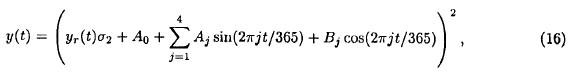
Prior to their use in DLTFN models, all the series were: <i>i)</i> Deseasonalized, by fitting them to the following function:</font></p>  	    <p align="center"><font face="verdana" size="2"><img src="/img/revistas/atm/v15n4/a4e1.jpg"></font></p>  	    <p align="justify"><font face="verdana" size="2">where only the yearly cycle and its first three harmonics have been included. No other period, apart from the annual, was found to be significant (Garrido and Garc&iacute;a, 1992). In the case of accumulated rainfall series, they were previously square root transformed in order to get an approximately normally distributed series (see Box and Cox, 1964; Delleur and Kavvas, 1978). Also, some peninsular pressure series were corrected for changes in location, <i>ii)</i> Detrended, by submitting each series to a homogeneity analysis (Mateos, 1993). In general, a linear trend was found to be enough to make the series stationary. <i>iii)</i> Finally, all the series were standardized, dividing them by their standard deviation. <a href="#t1">Table 1</a> shows the mean (<i>&#956;</i>) and the standard deviation (<i>&#963;</i><sub>0</sub>) of the original rainfall series, the mean (<i>&#956;</i><sub>1</sub>) and the standard deviation (<i>&#963;</i><sub>1</sub>) of the square root&#45;transformed rainfall series and the standard deviation (<i>&#963;</i><sub>2</sub>) of the deseasonalized series.</font></p>  	    <p>&nbsp;</p>  	    <p align="justify"><font face="verdana" size="2"><b>3. Discrete linear transfer function models</b></font></p>  	    <p align="justify"><font face="verdana" size="2"><i>a. Definition</i></font></p>  	    ]]></body>
<body><![CDATA[<p align="justify"><font face="verdana" size="2">Let <i>y(t)</i> and <i>x(t)</i> be a pair of series of data available at equally spaced intervals of time &#916;<i>t</i>, taken usually as 1, that could be considered as output and input of some dynamic system. <i>y(t)</i> and <i>x(t)</i> are supposedly related through a linear filter:</font></p>  	    <p align="center"><font face="verdana" size="2"><img src="/img/revistas/atm/v15n4/a4e2.jpg"></font></p>  	    <p align="justify"><font face="verdana" size="2">where <i>B</i> is the backshift operator <i>Bx</i>(<i>t</i>) <i>= x(t &#45;</i> 1). The polynomial <i>V(B)</i> = <i>v</i><sub>0</sub> <i>+ V</i><sub>1</sub><i>B + v</i><sub>2</sub><i>B + ...</i> is the transfer function of the filter. Weights <i>v</i><sub>0</sub> <i>,v</i><sub>1</sub><i>, ...</i> are called the input response of the system. The problem with equation (2) is that it has an infinite number of parameters. A parsimonious class of discrete linear transfer function models is given by (Box and Jenkins, 1976):</font></p>  	    <p align="center"><font face="verdana" size="2"><img src="/img/revistas/atm/v15n4/a4e3.jpg"></font></p>  	    <p align="justify"><font face="verdana" size="2">or</font></p>  	    <p align="center"><font face="verdana" size="2"><img src="/img/revistas/atm/v15n4/a4e4.jpg"></font></p>  	    <p align="justify"><font face="verdana" size="2">where <i>&#948;</i>(<i>B</i>) and <i>&#969;</i>(<i>B</i>) are polynomials of order <i>r</i> and <i>s</i> respectively. Equation (4) can be written as</font></p>  	    <p align="center"><font face="verdana" size="2"><img src="/img/revistas/atm/v15n4/a4e5.jpg"></font></p>  	    <p align="justify"><font face="verdana" size="2">Equating (2) and (5), produces a relation between <i>&#948;<sub>j</sub></i>, <i>&#969;<sub>j</sub></i>, and <i>v<sub>j</sub></i>. Noise has to be added to the input because the system is usually perturbed by unknown factors, not taken into account by the input <i>x(t),:</i></font></p>  	    <p align="center"><font face="verdana" size="2"><img src="/img/revistas/atm/v15n4/a4e6.jpg"></font></p>  	    ]]></body>
<body><![CDATA[<p align="justify"><font face="verdana" size="2">where <i>n(t)</i> represents the external noise which is usually shaped as an ARMA model,</font></p>  	    <p align="center"><font face="verdana" size="2"><img src="/img/revistas/atm/v15n4/a4e7.jpg"></font></p>  	    <p align="justify"><font face="verdana" size="2">&#934; <i>(B)</i> and &#936; <i>(B)</i> being two polynomials of orders <i>p</i> and <i>q</i> in the backshift operator <i>B,</i> and <i>a(t)</i> white noise. The final form of the DLTFN is</font></p>  	    <p align="center"><font face="verdana" size="2"><img src="/img/revistas/atm/v15n4/a4e8.jpg"></font></p>  	    <p><font face="verdana" size="2"><i>b.</i> Parameter <i>estimation</i></font></p>     <p align="justify"><font face="verdana" size="2">The parameter estimation is carried out in four steps. See Box and Jenkins (1976) for a full description of the fitting process.</font></p>  	    <p align="justify"><font face="verdana" size="2"><b>Identification of the model:</b> From the cross&#45;correlation function between the input series <i>x<sub>t</sub></i> and the output series <i>y<sub>t</sub></i>, weights <img src="/img/revistas/atm/v15n4/a4s3.jpg" align="absmiddle"> are estimated, from which the coefficients of the polynomials <img src="/img/revistas/atm/v15n4/a4s4.jpg" align="absmiddle"> and <img src="/img/revistas/atm/v15n4/a4s5.jpg" align="absmiddle"> are obtained for some selected values of the orders <i>r</i> and <i>s.</i> In this case, all possible combinations of 1 &#8804; r &#8804; 4 and 1 &#8804; s &#8804; 4, were tried keeping the one that gave minimum noise variance for subsequent analysis. Also, the roots of the <img src="/img/revistas/atm/v15n4/a4s4.jpg" align="absmiddle"> polynomial were evaluated in order to assure the stability of the model. In all cases, the minimum noise variance model was found to be stable.</font></p>  	    <p align="justify"><font face="verdana" size="2"><b>Identification of the noise:</b> An estimate <img src="/img/revistas/atm/v15n4/a4s6.jpg" align="absmiddle"> of the noise of the system is provided by subtracting the estimate <img src="/img/revistas/atm/v15n4/a4s7.jpg" align="absmiddle"> from the observed output of the system <i>y(t),</i> given by</font></p>  	    <p align="center"><font face="verdana" size="2"><img src="/img/revistas/atm/v15n4/a4e9.jpg"></font></p>  	    <p align="justify"><font face="verdana" size="2">Once the noise series has been obtained, it is ARMA modeled</font></p>  	    ]]></body>
<body><![CDATA[<p align="center"><font face="verdana" size="2"><img src="/img/revistas/atm/v15n4/a4e10.jpg"></font></p>  	    <p align="justify"><font face="verdana" size="2">where <i>a(t)</i> is white noise.</font></p>  	    <p align="justify"><font face="verdana" size="2"><b>Parameter estimation:</b> The final estimate of the parameters was obtained by fitting the series &#123;<i>x</i>(<i>t</i>),<i>y</i>(<i>t</i>)&#125; to Equation (8) by a non&#45;linear least squares method using the Levenberg&#45;Marquardt algorithm. The order of the model, i.e. <i>r</i>, <i>s</i>, <i>p</i>, <i>q</i> and the initial parameters for the non&#45;linear least squares algorithm are those obtained in previous steps. A 100(1&#45;&#945;)% confidence interval for the parameters was calculated according to Box and Jenkins (1976).</font></p>  	    <p align="center"><font face="verdana" size="2"><img src="/img/revistas/atm/v15n4/a4e11.jpg"></font></p>  	    <p align="justify"><font face="verdana" size="2">where &#948;&#946;<sub>i</sub> is the confidence interval for each parameter of the model, <i>&#963;</i><sub>a</sub><sup>2</sup> is the noise variance and C<i><sub>ii</sub></i> are the main diagonal elements of the covariance matrix (X'X)<sup>&#45;1</sup>, where X is the Jacobian <img src="/img/revistas/atm/v15n4/a4s9.jpg" align="absmiddle"> at the minimum, <i><img src="/img/revistas/atm/v15n4/a4s10.jpg" align="absmiddle"></i> is a two&#45;tailed 100<img src="/img/revistas/atm/v15n4/a4s8.jpg" align="absmiddle">% critical value of Student's <i>t</i>, and &#945; is taken to be 0.05.</font></p>  	    <p align="justify"><font face="verdana" size="2"><b>Checking the model:</b></font></p>  	    <p align="justify"><font face="verdana" size="2">The adequacy of the fit was tested by comparing the statistics (see Box and Jenkins (1976) for a thorough discussion)</font></p>  	    <p align="center"><font face="verdana" size="2"><img src="/img/revistas/atm/v15n4/a4e12.jpg"></font></p>  	    <p align="justify"><font face="verdana" size="2">against a &#967;<sup>2</sup> with <i>K &#45; m &#45; n</i> degrees of freedom, where <i>m</i>, <i>n</i> are the orders of the ARMA model fitted to the noise <i>n</i>(<i>t</i>) and <i>M = N &#45; p</i> is the number of values of <i>a</i>(<i>t</i>) that are actually available for computation, and statistics purposes</font></p>  	    <p align="center"><font face="verdana" size="2"><img src="/img/revistas/atm/v15n4/a4e13.jpg"></font></p>  	    ]]></body>
<body><![CDATA[<p align="justify"><font face="verdana" size="2">against a &#967;<sup>2</sup> with <i>K +</i> 1 <i>&#45;</i> (<i>r</i> + <i>s</i> + 1) degrees of freedom, where (<i>r</i> + <i>s +</i>1) is the number of parameters fitted in the DLTFN model. The <i>Q</i> test checks the adequacy of the noise model, and the <i>S</i> test the adequacy of the DLTFN model.</font></p>  	    <p>&nbsp;</p>  	    <p align="justify"><font face="verdana" size="2"><b>4. Forecasting</b></font></p>  	    <p align="justify"><font face="verdana" size="2">One of the main goals of time stochastic models is to forecast future values of the observed series <i>y</i>(<i>t</i>)<i>.</i> The method proposed by Box and Jenkins (1976) was followed. Using square brackets to denote conditional expectation at time t, and <img src="/img/revistas/atm/v15n4/a4s11.jpg" align="absmiddle"> and <img src="/img/revistas/atm/v15n4/a4s12.jpg" align="absmiddle"> to denote lead&#45;<i>l</i> forecasts of <i>y</i>(<i>t</i>) and <i>x</i>(<i>t</i>)<i>:</i></font></p> 	    <p align="center"><img src="/img/revistas/atm/v15n4/a4e14dibujo.jpg"></p>  	  	     <p align="justify"><font face="verdana" size="2">where</font></p>     <p align="center"><font face="verdana" size="2"><img src="/img/revistas/atm/v15n4/a4e141.jpg"></font></p>  	    <p align="justify"><font face="verdana" size="2">The <i>a</i>(<i>t</i>) series is calculated as <img src="/img/revistas/atm/v15n4/a4s13.jpg" align="absmiddle">, and the <img src="/img/revistas/atm/v15n4/a4s14.jpg" align="absmiddle"> series is obtained from the ARMA model fitted to the input series that was used for pre whitening. The variance of the lead&#45;1 forecast is given by</font></p>  	    <p align="center"><font face="verdana" size="2"><img src="/img/revistas/atm/v15n4/a4e15.jpg"></font></p>  	    <p>&nbsp;</p>  	    ]]></body>
<body><![CDATA[<p align="justify"><font face="verdana" size="2"><b>5. Results and discussion</b></font></p>  	    <p align="justify"><font face="verdana" size="2">For each accumulated rainfall series analyzed (one per observatory), three DLTFN models were obtained, one for each input series: LP, SST and SLP. An ARMA model was also fitted for comparison.
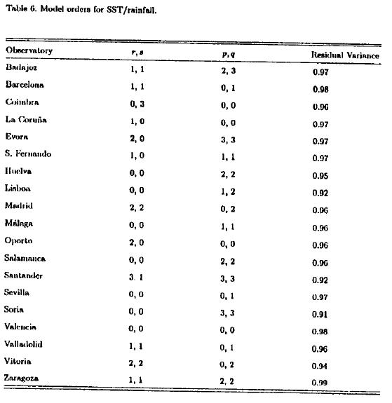
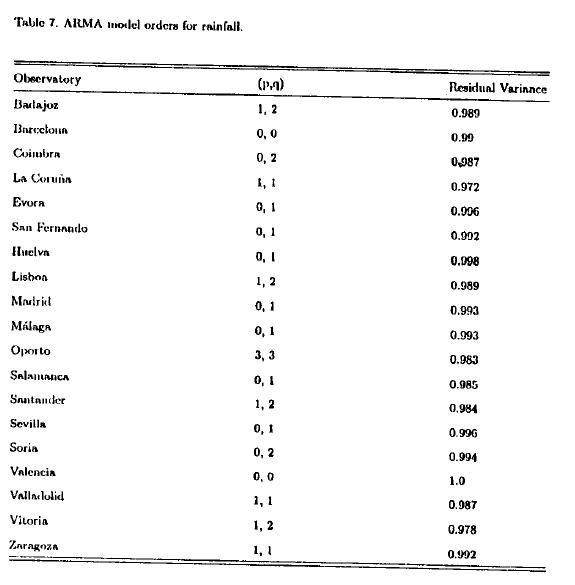
</font></p>  	    <p align="justify"><font face="verdana" size="2"><a href="#t4">Tables 4</a> to <a href="#t6">6</a> (<a href="#t5">5</a>) give the orders of the DLTFN models obtained, and <a href="#t7">Table 7</a> the orders of the ARMA models. The residual variance is also listed. <a href="#t8">Tables 8</a> to <a href="#t10">10</a> (<a href="#t9">9</a>) give the results of the <i>S</i> and <i>Q</i> tests. The tables present the values of <i>Q</i> and <i>S</i> obtained using Equations (12) and (13) with <i>K =</i> 100, the degree of freedom <i>v</i> and the <i>&#967;</i><sup>2</sup> critical value at a 5% level of significance. The model is not rejected when <i>Q, S &#8804;</i> <i>&#967;</i><sup>2</sup>. According to these tables, the models are rejected in only a few cases &#91;San Fernando, Huelva (Q test, LP/rainfall), Barcelona (Q test, SST/Rainfall)&#93;.</font></p>  	    <p align="center"><font face="verdana" size="2"><a name="t4"></a></font></p>  	    <p align="center"><font face="verdana" size="2"><img src="/img/revistas/atm/v15n4/a4t4.jpg"></font></p>  	    <p align="center"><font face="verdana" size="2"><a name="t5"></a></font></p>  	    <p align="center"><font face="verdana" size="2"><img src="/img/revistas/atm/v15n4/a4t5.jpg"></font></p>  	    <p align="center"><font face="verdana" size="2"><a name="t6"></a></font></p>  	    <p align="center"><font face="verdana" size="2"><img src="/img/revistas/atm/v15n4/a4t6.jpg"></font></p>  	    <p align="center"><font face="verdana" size="2"><a name="t7"></a></font></p>  	    ]]></body>
<body><![CDATA[<p align="center"><font face="verdana" size="2"><img src="/img/revistas/atm/v15n4/a4t7.jpg"></font></p>  	    <p align="center"><font face="verdana" size="2"><a name="t8"></a></font></p>  	    <p align="center"><font face="verdana" size="2"><img src="/img/revistas/atm/v15n4/a4t8.jpg"></font></p>  	    <p align="center"><font face="verdana" size="2"><a name="t9"></a></font></p>  	    <p align="center"><font face="verdana" size="2"><img src="/img/revistas/atm/v15n4/a4t9.jpg"></font></p>  	    <p align="center"><font face="verdana" size="2"><a name="t10"></a></font></p>  	    <p align="center"><font face="verdana" size="2"><img src="/img/revistas/atm/v15n4/a4t10.jpg"></font></p>  	    <p align="justify"><font face="verdana" size="2">
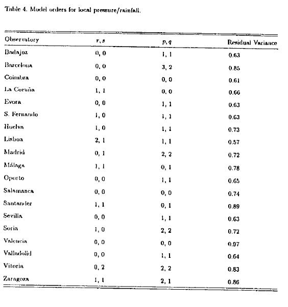
The best fit, measured by the variance reduction, is obtained when LP is the input variable, followed by SLP. The worst is obtained for the SST input series. In all cases, the variance reduction obtained with the DLTFN models is greater than the reduction in variance obtained with the ARMA models.</font></p>  	    <p align="justify"><font face="verdana" size="2">
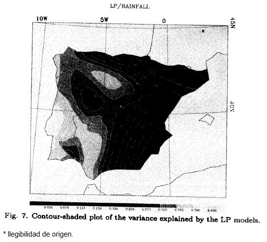
For the LP/rainfall models the explained variance is greater in observatories near the Atlantic coast. In moving away from the Atlantic, the explained variance decreases. The worst case (in terms of the explained variance) is obtained for Barcelona and Valencia on the Mediterranean coast, and for Santander and Vitoria near the Bay of Biscay. This is clearly seen in the contour plot of the explained variance displayed in <a href="#f7">Figure 7</a>.</font></p>  	    <p align="center"><font face="verdana" size="2"><a name="f7"></a></font></p>  	    ]]></body>
<body><![CDATA[<p align="center"><font face="verdana" size="2"><img src="/img/revistas/atm/v15n4/a4f7.jpg"></font></p>  	    <p align="justify"><font face="verdana" size="2">With reference to the SLP/rainfall models, <a href="#f8">Figure 8</a> shows a contour plot of the explained variance.</font></p>  	    <p align="center"><font face="verdana" size="2"><a name="f8"></a></font></p>  	    <p align="center"><font face="verdana" size="2"><img src="/img/revistas/atm/v15n4/a4f8.jpg"></font></p>  	    <p align="justify"><font face="verdana" size="2">
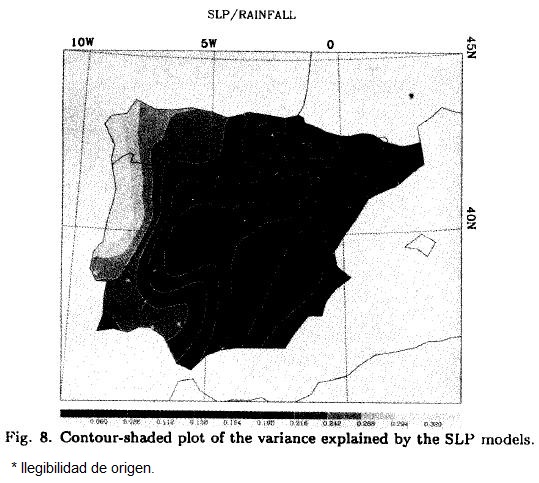
As before, the models work better for the observatories situated in the northwestern part of the Iberian Peninsula, decreasing in quality of performance as approaching the Mediterranean coast.</font></p>  	    <p align="justify"><font face="verdana" size="2">For the SST/rainfall models, <a href="#f9">Figure 9</a> presents the results of the explained variance. The explained variance is so low that there seems to be no definite region where the models work better than in others (except perhaps for Soria, which is believed to have no climatological significance).</font></p>  	    <p align="center"><font face="verdana" size="2"><a name="f9"></a></font></p>  	    <p align="center"><font face="verdana" size="2"><img src="/img/revistas/atm/v15n4/a4f9.jpg"></font></p>  	    <p align="justify"><font face="verdana" size="2">As <a href="#t4">Table 4</a> shows, most of the models present either a zeroth&#45;order polynomial <i>&#969;</i>(<i>B</i>) or an <i>&#969;</i>(<i>B</i>) with its first&#45; order coefficient <i>&#969;</i><sub>1</sub> much smaller than the zeroth&#45;order coefficient <i>&#969;</i><sub>0</sub><i>.</i> This means that the models are really diagnostic rather than prognostic, and their forecasting ability will really be that of the ARMA models fitted to the input series <i>x</i><sub>t</sub><i>.</i> Because in practically all the cases analyzed (LP, SLP and SST) these ARMA models behave as white noise, the forecasting models only for the most favorable cases should be develped, that is, when the LP are the input series, and using the models as diagnostic rather than prognostic models. Hence, we shall limit the research to the observational period, to using a lead&#45;1 forecast, and to using the observed pressure value instead of the predicted value when applying Equation (14). In order to compare the forecast value with the observed one, the path followed to the normalization has to be reversed, i.e., Equation (1) must be replaced by</font></p>  	    <p align="center"><font face="verdana" size="2"><img src="/img/revistas/atm/v15n4/a4e16.jpg"></font></p>  	    ]]></body>
<body><![CDATA[<p align="justify"><font face="verdana" size="2">where <i>y<sub>r</sub></i>(<i>t</i>) is the forecast value given by the DLTFN model using (14) and <i>&#963;</i><sub>2</sub> is the standard deviation of the deseasonalized rainfall series. The square has been added because the rainfall series were previously square root transformed. A 100(1&#45;&#945;)% confidence interval for the forecast value was calculated as</font></p>  	    <p align="center"><font face="verdana" size="2"><img src="/img/revistas/atm/v15n4/a4e17.jpg"></font></p>  	    <p align="justify"><font face="verdana" size="2">where <img src="/img/revistas/atm/v15n4/a4s15.jpg" align="absmiddle"> is a two&#45;tailed 100&#945;% critical value of Student's t, and &#945; is taken to be 0.05. <i>V</i>(1) is the variance of the lead&#45;1 forecast. <a href="/img/revistas/atm/v15n4/a4f10.jpg" target="_blank">Figure 10</a> shows the results obtained at some observatories. Filled circles show the observed values while open circles indicate the forecast ones. The error bars are the confidence intervals calculated using (17). As the figure shows, the forecast values are not much too different from the observed ones, but the error bars are quite large due to the high variance left unexplained. Obviously, observatories with smaller lead&#45;1 forecast variance show smaller error bars. This is easily seen by comparing the results of Valladolid or Madrid with those of La Coru&ntilde;a or Lisboa.</font></p>  	    <p align="justify"><font face="verdana" size="2">In order to better understand the results, we must analyze the origin of precipitation over the Iberian peninsula. The classical works on this topic are those of Lin&eacute;s (1981), who analyzed the perturbations and the associated rainfall that affect the Iberian Peninsula, Font (1983), who made a classification of the different weather types that affect the Peninsula, and more recently Marroquin et al. (1995), who analyzed the synoptic situations that seem responsible for the daily rainfall over Badajoz (one of the observatories studied, and a typical example of these results) and Ribalaygua and Bor&eacute;n (1996), who analyzed the relationship between the daily synoptic situations and the daily rainfall patterns over the Peninsula.</font></p>  	    <p align="justify"><font face="verdana" size="2">According to the results obtained by the aforementioned authors, a good deal of the rainfall over most of the Iberian Peninsula is related to the passages of fronts, moving eastward, with the associated low pressure center located in or near boxes #176, 177 and 212. This kind of synoptic situation is particularly important for the western two&#45;thirds of the Iberian Peninsula, whereas the Mediterranean coast rainfall has a major convective and orographic origin with westerly flow and a low located in the Gulf of Genova (Catalonian rainfall) or the Gulf of Cadiz (Valencia rainfall). Also a good deal of the rainfall over the Gulf of Biscay coast is associated with a northern flow with high pressures west of the British Isles, and a low in the Gulf of Genova. Our results agree fairly well with the above in that:</font></p>  	    <blockquote> 		    <p align="justify"><font face="verdana" size="2">&bull;&nbsp;The LP/rainfall models work well for the western part of the country (rainfall due to frontal passage).</font></p>  		    <p align="justify"><font face="verdana" size="2">&bull;&nbsp;The SLP/rainfall models work well for the western part of the country (lows located to the west/northwest of the Peninsula).</font></p> 	</blockquote>  	    <p>&nbsp;</p>  	    <p align="justify"><font face="verdana" size="2"><b>6. Summary and conclusions</b></font></p>  	    ]]></body>
<body><![CDATA[<p align="justify"><font face="verdana" size="2">In order to try to improve the results given by ARMA modeling of monthly accumulated rainfall series, a Discrete Linear Transfer Function Noise model was used, thus introducing new information given by an external variable &#45; in this case, North Atlantic SST, SLP and Local Pressure, LP.</font></p>  	    <p align="justify"><font face="verdana" size="2">The preliminary analysis shows that there is a small but significant relation between SST measured along a belt from 10 to 20&deg;N and the rainfall measured at observatories on the west and southwest of the Iberian Peninsula. This relation is much greater when the SLP data are taken as input variables. In this case, the highest correlation North Atlantic zone stretches from 30 to 50&deg;N and lies just to the west of the Iberian Peninsula.</font></p>  	    <p align="justify"><font face="verdana" size="2">In all cases analyzed, the performance of the DLTFN models, measured by the explained variance of the rainfall series, is better than that of ARMA models. The model that 'works' best is the one where the input variables are LP, followed by SLP, and SST.</font></p>  	    <p align="justify"><font face="verdana" size="2">In most of the models, the first coefficient <i>&#969;</i><sub>1</sub> of the polynomial <i>&#969;</i>(<i>B</i>) is either zero or much smaller than the zeroth&#45;order coefficient <i>&#969;</i><sub>0</sub>, which means that the models are diagnostic rather than prognostic. We therefore used them as a prognostic tool, keeping our 'forecasting' within the observational period.</font></p>  	    <p>&nbsp;</p>  	    <p align="justify"><font face="verdana" size="2"><b>Acknowledgements</b></font></p>  	    <p align="justify"><font face="verdana" size="2">Thanks are due to the Instituto Nacional de Meteorolog&iacute;a of Spain for providing us with rainfall and local pressure data, and to the Spanish CICYT for their financial support, project number CLI96&#45;1871&#45;C04&#45;03. Thanks are also due to the anonymous reviewers for their useful comments.</font></p>  	    <p>&nbsp;</p>  	    <p align="justify"><font face="verdana" size="2"><b>REFERENCES</b></font></p>  	    <!-- ref --><p align="justify"><font face="verdana" size="2">Barnett, T. P., 1984. Statistical prediction of seasonal air temperature over Eurasia. <i>Tellus,</i> 36A, 132&#45;146.    &nbsp;&nbsp;&nbsp;&nbsp;&nbsp;&nbsp;&nbsp;&nbsp;[&#160;<a href="javascript:void(0);" onclick="javascript: window.open('/scielo.php?script=sci_nlinks&ref=1251876&pid=S0187-6236200200040000400001&lng=','','width=640,height=500,resizable=yes,scrollbars=1,menubar=yes,');">Links</a>&#160;]<!-- end-ref --></font></p>  	    <!-- ref --><p align="justify"><font face="verdana" size="2">Bennett, R.J., 1979. Spatial Time Series. Pion Limited. London.    &nbsp;&nbsp;&nbsp;&nbsp;&nbsp;&nbsp;&nbsp;&nbsp;[&#160;<a href="javascript:void(0);" onclick="javascript: window.open('/scielo.php?script=sci_nlinks&ref=1251878&pid=S0187-6236200200040000400002&lng=','','width=640,height=500,resizable=yes,scrollbars=1,menubar=yes,');">Links</a>&#160;]<!-- end-ref --></font></p>  	    <!-- ref --><p align="justify"><font face="verdana" size="2">Box, G. E. P. and D. R. Cox, 1964. An analysis of transformations. <i>J. Roy. Statis. Soc., Ser. B,</i> 26, 211&#45;252.    &nbsp;&nbsp;&nbsp;&nbsp;&nbsp;&nbsp;&nbsp;&nbsp;[&#160;<a href="javascript:void(0);" onclick="javascript: window.open('/scielo.php?script=sci_nlinks&ref=1251880&pid=S0187-6236200200040000400003&lng=','','width=640,height=500,resizable=yes,scrollbars=1,menubar=yes,');">Links</a>&#160;]<!-- end-ref --></font></p>  	    <!-- ref --><p align="justify"><font face="verdana" size="2">Box, G. E. P. and G. M. Jenkins, 1976. Time Series Analysis: Forecasting and Control (rev.). Holden&#45;Day. San Francisco.    &nbsp;&nbsp;&nbsp;&nbsp;&nbsp;&nbsp;&nbsp;&nbsp;[&#160;<a href="javascript:void(0);" onclick="javascript: window.open('/scielo.php?script=sci_nlinks&ref=1251882&pid=S0187-6236200200040000400004&lng=','','width=640,height=500,resizable=yes,scrollbars=1,menubar=yes,');">Links</a>&#160;]<!-- end-ref --></font></p>  	    <!-- ref --><p align="justify"><font face="verdana" size="2">Delleur, J. M. and M. L. Kavvas, 1978. Stochastic models for monthly rainfall forecasting and synthetic generation. <i>J. Appl. Meteor.,</i> 17<i>,</i> 1528&#45;1536.    &nbsp;&nbsp;&nbsp;&nbsp;&nbsp;&nbsp;&nbsp;&nbsp;[&#160;<a href="javascript:void(0);" onclick="javascript: window.open('/scielo.php?script=sci_nlinks&ref=1251884&pid=S0187-6236200200040000400005&lng=','','width=640,height=500,resizable=yes,scrollbars=1,menubar=yes,');">Links</a>&#160;]<!-- end-ref --></font></p>  	    <!-- ref --><p align="justify"><font face="verdana" size="2">Efrom, B. and R. J. Tibshirani, 1993. An Introduction to the Bootstrap. Chapman and Hall. New York.    &nbsp;&nbsp;&nbsp;&nbsp;&nbsp;&nbsp;&nbsp;&nbsp;[&#160;<a href="javascript:void(0);" onclick="javascript: window.open('/scielo.php?script=sci_nlinks&ref=1251886&pid=S0187-6236200200040000400006&lng=','','width=640,height=500,resizable=yes,scrollbars=1,menubar=yes,');">Links</a>&#160;]<!-- end-ref --></font></p>  	    <!-- ref --><p align="justify"><font face="verdana" size="2">Folland, C. K., T. N. Palmer and D. E. Parker, 1986. Sahel rainfall and the worldwide sea temperatures 1901&#45;85. <i>Nature,</i> 320, 602&#45;607.    &nbsp;&nbsp;&nbsp;&nbsp;&nbsp;&nbsp;&nbsp;&nbsp;[&#160;<a href="javascript:void(0);" onclick="javascript: window.open('/scielo.php?script=sci_nlinks&ref=1251888&pid=S0187-6236200200040000400007&lng=','','width=640,height=500,resizable=yes,scrollbars=1,menubar=yes,');">Links</a>&#160;]<!-- end-ref --></font></p>  	    <!-- ref --><p align="justify"><font face="verdana" size="2">Font, I., 1983. Climatolog&iacute;a de Espa&ntilde;a y Portugal, Instituto Nacional de Meteorolog&iacute;a, Madrid, Spain.    &nbsp;&nbsp;&nbsp;&nbsp;&nbsp;&nbsp;&nbsp;&nbsp;[&#160;<a href="javascript:void(0);" onclick="javascript: window.open('/scielo.php?script=sci_nlinks&ref=1251890&pid=S0187-6236200200040000400008&lng=','','width=640,height=500,resizable=yes,scrollbars=1,menubar=yes,');">Links</a>&#160;]<!-- end-ref --></font></p>  	    <!-- ref --><p align="justify"><font face="verdana" size="2">Fontaine, B., S. Janicot and V. Moron, 1995. Rainfall anomaly patterns and wind field signals over West Africa in August (1958&#45;1989). <i>J. Climate,</i> 8, 1503&#45;1510.    &nbsp;&nbsp;&nbsp;&nbsp;&nbsp;&nbsp;&nbsp;&nbsp;[&#160;<a href="javascript:void(0);" onclick="javascript: window.open('/scielo.php?script=sci_nlinks&ref=1251892&pid=S0187-6236200200040000400009&lng=','','width=640,height=500,resizable=yes,scrollbars=1,menubar=yes,');">Links</a>&#160;]<!-- end-ref --></font></p>  	    <!-- ref --><p align="justify"><font face="verdana" size="2">Garrido, J. and J. A. Garc&iacute;a, 1992. Periodic signals in Spanish monthly precipitation data. <i>Theor. Appl. Clirnatol.,</i> 45, 97&#45;106.    &nbsp;&nbsp;&nbsp;&nbsp;&nbsp;&nbsp;&nbsp;&nbsp;[&#160;<a href="javascript:void(0);" onclick="javascript: window.open('/scielo.php?script=sci_nlinks&ref=1251894&pid=S0187-6236200200040000400010&lng=','','width=640,height=500,resizable=yes,scrollbars=1,menubar=yes,');">Links</a>&#160;]<!-- end-ref --></font></p>  	    <!-- ref --><p align="justify"><font face="verdana" size="2">Garrido, J. and J. A. Garc&iacute;a, 1993. Aplicaci&oacute;n de los procesos de autoregresivos&#45;media m&oacute;vil para modelizar series temporales de precipitaci&oacute;n en la Espa&ntilde;a peninsular. <i>Anales de F&iacute;sica,</i> 89, 50&#45;56.    &nbsp;&nbsp;&nbsp;&nbsp;&nbsp;&nbsp;&nbsp;&nbsp;[&#160;<a href="javascript:void(0);" onclick="javascript: window.open('/scielo.php?script=sci_nlinks&ref=1251896&pid=S0187-6236200200040000400011&lng=','','width=640,height=500,resizable=yes,scrollbars=1,menubar=yes,');">Links</a>&#160;]<!-- end-ref --></font></p>  	    <!-- ref --><p align="justify"><font face="verdana" size="2">Hastenrath, S., L. Greischar and J. van Heerden, 1995. Prediction of summer rainfall over South Africa. <i>J. Climate,</i> 8, 1511&#45;1518.    &nbsp;&nbsp;&nbsp;&nbsp;&nbsp;&nbsp;&nbsp;&nbsp;[&#160;<a href="javascript:void(0);" onclick="javascript: window.open('/scielo.php?script=sci_nlinks&ref=1251898&pid=S0187-6236200200040000400012&lng=','','width=640,height=500,resizable=yes,scrollbars=1,menubar=yes,');">Links</a>&#160;]<!-- end-ref --></font></p>      <!-- ref --><p align="justify"><font face="verdana" size="2">Kahl, J. D., D. J. Charlevoix, N. A. Zaitseva, R. C. Schnell and M. C. Serreze, 1993. Absence of evidence for greenhouse warming over the Arctic Ocean in the past 40 years. <i>Nature,</i> 361, 335&#45;337.    &nbsp;&nbsp;&nbsp;&nbsp;&nbsp;&nbsp;&nbsp;&nbsp;[&#160;<a href="javascript:void(0);" onclick="javascript: window.open('/scielo.php?script=sci_nlinks&ref=1251900&pid=S0187-6236200200040000400013&lng=','','width=640,height=500,resizable=yes,scrollbars=1,menubar=yes,');">Links</a>&#160;]<!-- end-ref --></font></p>  	    <!-- ref --><p align="justify"><font face="verdana" size="2">Katz, R. W. and R. H. Skaggs, 1981. On the use of autoregressive&#45;moving average processes to model meteorological times series. <i>Mon. Wea. Rev.,</i> 109, 479&#45;484.    &nbsp;&nbsp;&nbsp;&nbsp;&nbsp;&nbsp;&nbsp;&nbsp;[&#160;<a href="javascript:void(0);" onclick="javascript: window.open('/scielo.php?script=sci_nlinks&ref=1251902&pid=S0187-6236200200040000400014&lng=','','width=640,height=500,resizable=yes,scrollbars=1,menubar=yes,');">Links</a>&#160;]<!-- end-ref --></font></p>  	    <!-- ref --><p align="justify"><font face="verdana" size="2">Lin&eacute;s, A., 1981. Perturbaciones t&iacute;picas que afectan a la Pen&iacute;nsula Ib&eacute;rica y precipitaciones asociadas. Instituto Nacional de Meteorolog&iacute;a de Espa&ntilde;a, Madrid.    &nbsp;&nbsp;&nbsp;&nbsp;&nbsp;&nbsp;&nbsp;&nbsp;[&#160;<a href="javascript:void(0);" onclick="javascript: window.open('/scielo.php?script=sci_nlinks&ref=1251904&pid=S0187-6236200200040000400015&lng=','','width=640,height=500,resizable=yes,scrollbars=1,menubar=yes,');">Links</a>&#160;]<!-- end-ref --></font></p>  	    <!-- ref --><p align="justify"><font face="verdana" size="2">Lorente, J. M., 1985. La variabilidad de las precipitaciones atmosf&eacute;ricas sobre la Espa&ntilde;a peninsular. <i>Revista de Geof&iacute;sica XIV,</i> Madrid.    &nbsp;&nbsp;&nbsp;&nbsp;&nbsp;&nbsp;&nbsp;&nbsp;[&#160;<a href="javascript:void(0);" onclick="javascript: window.open('/scielo.php?script=sci_nlinks&ref=1251906&pid=S0187-6236200200040000400016&lng=','','width=640,height=500,resizable=yes,scrollbars=1,menubar=yes,');">Links</a>&#160;]<!-- end-ref --></font></p>  	    <!-- ref --><p align="justify"><font face="verdana" size="2">Marroquin A., J. A. Garc&iacute;a, J. Garrido and V. L. Mateos, 1995. Neymann&#45;Scott cluster model for daily rainfall processes in Lower Extremadura (Spain). Rainfall generating mechanisms. <i>Theor. Appl. Clirnatol.</i> 52, 183&#45;195.    &nbsp;&nbsp;&nbsp;&nbsp;&nbsp;&nbsp;&nbsp;&nbsp;[&#160;<a href="javascript:void(0);" onclick="javascript: window.open('/scielo.php?script=sci_nlinks&ref=1251908&pid=S0187-6236200200040000400017&lng=','','width=640,height=500,resizable=yes,scrollbars=1,menubar=yes,');">Links</a>&#160;]<!-- end-ref --></font></p>  	    <!-- ref --><p align="justify"><font face="verdana" size="2">Mateos, V. L., 1993. Modelos de Funci&oacute;n de Transferencia para series de precipitaci&oacute;n en la pen&iacute;nsula Ib&eacute;rica, Ph. D. Thesis, Universidad de Extremadura, Espa&ntilde;a.    &nbsp;&nbsp;&nbsp;&nbsp;&nbsp;&nbsp;&nbsp;&nbsp;[&#160;<a href="javascript:void(0);" onclick="javascript: window.open('/scielo.php?script=sci_nlinks&ref=1251910&pid=S0187-6236200200040000400018&lng=','','width=640,height=500,resizable=yes,scrollbars=1,menubar=yes,');">Links</a>&#160;]<!-- end-ref --></font></p>  	    <!-- ref --><p align="justify"><font face="verdana" size="2">Meehl G. A. and H. van Loon, 1979. The seesaw in winter temperatures between Greenland and northern Europe. Part III: Teleconnections with Lower Latitudes. <i>Mon. Wea. Rev.,</i> 107, 1095&#45;1106.    &nbsp;&nbsp;&nbsp;&nbsp;&nbsp;&nbsp;&nbsp;&nbsp;[&#160;<a href="javascript:void(0);" onclick="javascript: window.open('/scielo.php?script=sci_nlinks&ref=1251912&pid=S0187-6236200200040000400019&lng=','','width=640,height=500,resizable=yes,scrollbars=1,menubar=yes,');">Links</a>&#160;]<!-- end-ref --></font></p>  	    <!-- ref --><p align="justify"><font face="verdana" size="2">Nicholls, N., 1989. Sea surface temperature and Australian winter rainfall. <i>J. of Climate,</i> 2, 965&#45;973.    &nbsp;&nbsp;&nbsp;&nbsp;&nbsp;&nbsp;&nbsp;&nbsp;[&#160;<a href="javascript:void(0);" onclick="javascript: window.open('/scielo.php?script=sci_nlinks&ref=1251914&pid=S0187-6236200200040000400020&lng=','','width=640,height=500,resizable=yes,scrollbars=1,menubar=yes,');">Links</a>&#160;]<!-- end-ref --></font></p>  	    <!-- ref --><p align="justify"><font face="verdana" size="2">Ratcliffe, R. A. S. and R. Murray, 1970. New lag associations between North Atlantic sea temperature and European pressure applied to long&#45;range weather forecasting. <i>Quart. J. Roy. Meteor. Soc.</i> 96, 226&#45;246.    &nbsp;&nbsp;&nbsp;&nbsp;&nbsp;&nbsp;&nbsp;&nbsp;[&#160;<a href="javascript:void(0);" onclick="javascript: window.open('/scielo.php?script=sci_nlinks&ref=1251916&pid=S0187-6236200200040000400021&lng=','','width=640,height=500,resizable=yes,scrollbars=1,menubar=yes,');">Links</a>&#160;]<!-- end-ref --></font></p>  	    <!-- ref --><p align="justify"><font face="verdana" size="2">Ribalaygua, J. and R. Bor&eacute;n, 1996. Clasificaci&oacute;n de Patrones de Precipitaci&oacute;n Diaria Sobre la Espa&ntilde;a Peninsular y Bale&aacute;rica, Informe N&deg;3, Servicio de An&aacute;lisis e Investigaci&oacute;n del Clima, Instituto Nacional de Meteorolog&iacute;a, Spain.    &nbsp;&nbsp;&nbsp;&nbsp;&nbsp;&nbsp;&nbsp;&nbsp;[&#160;<a href="javascript:void(0);" onclick="javascript: window.open('/scielo.php?script=sci_nlinks&ref=1251918&pid=S0187-6236200200040000400022&lng=','','width=640,height=500,resizable=yes,scrollbars=1,menubar=yes,');">Links</a>&#160;]<!-- end-ref --></font></p>  	    <!-- ref --><p align="justify"><font face="verdana" size="2">Rowntree, P. R., 1976. Response of the atmosphere to a tropical Atlantic Ocean temperature anomaly. <i>Quart. J. R. Met. Soc.,</i> 102, 607&#45;625.    &nbsp;&nbsp;&nbsp;&nbsp;&nbsp;&nbsp;&nbsp;&nbsp;[&#160;<a href="javascript:void(0);" onclick="javascript: window.open('/scielo.php?script=sci_nlinks&ref=1251920&pid=S0187-6236200200040000400023&lng=','','width=640,height=500,resizable=yes,scrollbars=1,menubar=yes,');">Links</a>&#160;]<!-- end-ref --></font></p>  	    <!-- ref --><p align="justify"><font face="verdana" size="2">Woodruff, S. D., R. J. Slutz, R. J. Jenne and P. M. Steurer, 1987. A comprehensive ocean&#45;atmosphere data set. <i>Bull. Amer. Meteor. Soc.,</i> 68, 1239&#45;1250.    &nbsp;&nbsp;&nbsp;&nbsp;&nbsp;&nbsp;&nbsp;&nbsp;[&#160;<a href="javascript:void(0);" onclick="javascript: window.open('/scielo.php?script=sci_nlinks&ref=1251922&pid=S0187-6236200200040000400024&lng=','','width=640,height=500,resizable=yes,scrollbars=1,menubar=yes,');">Links</a>&#160;]<!-- end-ref --></font></p>      ]]></body><back>
<ref-list>
<ref id="B1">
<nlm-citation citation-type="journal">
<person-group person-group-type="author">
<name>
<surname><![CDATA[Barnett]]></surname>
<given-names><![CDATA[T. P.]]></given-names>
</name>
</person-group>
<article-title xml:lang="en"><![CDATA[Statistical prediction of seasonal air temperature over Eurasia]]></article-title>
<source><![CDATA[Tellus]]></source>
<year>1984</year>
<volume>36A</volume>
<page-range>132-146</page-range></nlm-citation>
</ref>
<ref id="B2">
<nlm-citation citation-type="book">
<person-group person-group-type="author">
<name>
<surname><![CDATA[Bennett]]></surname>
<given-names><![CDATA[R.J.]]></given-names>
</name>
</person-group>
<source><![CDATA[Spatial Time Series]]></source>
<year>1979</year>
<publisher-loc><![CDATA[London ]]></publisher-loc>
<publisher-name><![CDATA[Pion Limited]]></publisher-name>
</nlm-citation>
</ref>
<ref id="B3">
<nlm-citation citation-type="journal">
<person-group person-group-type="author">
<name>
<surname><![CDATA[Box]]></surname>
<given-names><![CDATA[G. E. P.]]></given-names>
</name>
<name>
<surname><![CDATA[Cox]]></surname>
<given-names><![CDATA[D. R.]]></given-names>
</name>
</person-group>
<article-title xml:lang="en"><![CDATA[An analysis of transformations]]></article-title>
<source><![CDATA[J. Roy. Statis. Soc., Ser. B]]></source>
<year>1964</year>
<volume>26</volume>
<page-range>211-252</page-range></nlm-citation>
</ref>
<ref id="B4">
<nlm-citation citation-type="book">
<person-group person-group-type="author">
<name>
<surname><![CDATA[Box]]></surname>
<given-names><![CDATA[G. E. P.]]></given-names>
</name>
<name>
<surname><![CDATA[Jenkins]]></surname>
<given-names><![CDATA[G. M.]]></given-names>
</name>
</person-group>
<source><![CDATA[Time Series Analysis: Forecasting and Control (rev.)]]></source>
<year>1976</year>
<publisher-loc><![CDATA[San Francisco ]]></publisher-loc>
<publisher-name><![CDATA[Holden-Day]]></publisher-name>
</nlm-citation>
</ref>
<ref id="B5">
<nlm-citation citation-type="journal">
<person-group person-group-type="author">
<name>
<surname><![CDATA[Delleur]]></surname>
<given-names><![CDATA[J. M.]]></given-names>
</name>
<name>
<surname><![CDATA[Kavvas]]></surname>
<given-names><![CDATA[M. L.]]></given-names>
</name>
</person-group>
<article-title xml:lang="en"><![CDATA[Stochastic models for monthly rainfall forecasting and synthetic generation]]></article-title>
<source><![CDATA[J. Appl. Meteor.]]></source>
<year>1978</year>
<volume>17</volume>
<page-range>1528-1536</page-range></nlm-citation>
</ref>
<ref id="B6">
<nlm-citation citation-type="book">
<person-group person-group-type="author">
<name>
<surname><![CDATA[Efrom]]></surname>
<given-names><![CDATA[B.]]></given-names>
</name>
<name>
<surname><![CDATA[Tibshirani]]></surname>
<given-names><![CDATA[R. J.]]></given-names>
</name>
</person-group>
<source><![CDATA[An Introduction to the Bootstrap]]></source>
<year>1993</year>
<publisher-loc><![CDATA[New York ]]></publisher-loc>
<publisher-name><![CDATA[Chapman and Hall]]></publisher-name>
</nlm-citation>
</ref>
<ref id="B7">
<nlm-citation citation-type="journal">
<person-group person-group-type="author">
<name>
<surname><![CDATA[Folland]]></surname>
<given-names><![CDATA[C. K.]]></given-names>
</name>
<name>
<surname><![CDATA[Palmer]]></surname>
<given-names><![CDATA[T. N.]]></given-names>
</name>
<name>
<surname><![CDATA[Parker]]></surname>
<given-names><![CDATA[D. E.]]></given-names>
</name>
</person-group>
<article-title xml:lang="en"><![CDATA[Sahel rainfall and the worldwide sea temperatures 1901-85]]></article-title>
<source><![CDATA[Nature]]></source>
<year>1986</year>
<volume>320</volume>
<page-range>602-607</page-range></nlm-citation>
</ref>
<ref id="B8">
<nlm-citation citation-type="book">
<person-group person-group-type="author">
<name>
<surname><![CDATA[Font]]></surname>
<given-names><![CDATA[I.]]></given-names>
</name>
</person-group>
<source><![CDATA[Climatología de España y Portugal]]></source>
<year>1983</year>
<publisher-loc><![CDATA[Madrid ]]></publisher-loc>
<publisher-name><![CDATA[Instituto Nacional de Meteorología]]></publisher-name>
</nlm-citation>
</ref>
<ref id="B9">
<nlm-citation citation-type="journal">
<person-group person-group-type="author">
<name>
<surname><![CDATA[Fontaine]]></surname>
<given-names><![CDATA[B.]]></given-names>
</name>
<name>
<surname><![CDATA[Janicot]]></surname>
<given-names><![CDATA[S.]]></given-names>
</name>
<name>
<surname><![CDATA[Moron]]></surname>
<given-names><![CDATA[V.]]></given-names>
</name>
</person-group>
<article-title xml:lang="en"><![CDATA[Rainfall anomaly patterns and wind field signals over West Africa in August (1958-1989)]]></article-title>
<source><![CDATA[J. Climate]]></source>
<year>1995</year>
<volume>8</volume>
<page-range>1503-1510</page-range></nlm-citation>
</ref>
<ref id="B10">
<nlm-citation citation-type="journal">
<person-group person-group-type="author">
<name>
<surname><![CDATA[Garrido]]></surname>
<given-names><![CDATA[J.]]></given-names>
</name>
<name>
<surname><![CDATA[García]]></surname>
<given-names><![CDATA[J. A.]]></given-names>
</name>
</person-group>
<article-title xml:lang="en"><![CDATA[Periodic signals in Spanish monthly precipitation data]]></article-title>
<source><![CDATA[Theor. Appl. Clirnatol.]]></source>
<year>1992</year>
<volume>45</volume>
<page-range>97-106</page-range></nlm-citation>
</ref>
<ref id="B11">
<nlm-citation citation-type="journal">
<person-group person-group-type="author">
<name>
<surname><![CDATA[Garrido]]></surname>
<given-names><![CDATA[J.]]></given-names>
</name>
<name>
<surname><![CDATA[García]]></surname>
<given-names><![CDATA[J. A.]]></given-names>
</name>
</person-group>
<article-title xml:lang="es"><![CDATA[Aplicación de los procesos de autoregresivos-media móvil para modelizar series temporales de precipitación en la España peninsular]]></article-title>
<source><![CDATA[Anales de Física]]></source>
<year>1993</year>
<volume>89</volume>
<page-range>50-56</page-range></nlm-citation>
</ref>
<ref id="B12">
<nlm-citation citation-type="journal">
<person-group person-group-type="author">
<name>
<surname><![CDATA[Hastenrath]]></surname>
<given-names><![CDATA[S.]]></given-names>
</name>
<name>
<surname><![CDATA[Greischar]]></surname>
<given-names><![CDATA[L.]]></given-names>
</name>
<name>
<surname><![CDATA[van Heerden]]></surname>
<given-names><![CDATA[J.]]></given-names>
</name>
</person-group>
<article-title xml:lang="en"><![CDATA[Prediction of summer rainfall over South Africa]]></article-title>
<source><![CDATA[J. Climate]]></source>
<year>1995</year>
<volume>8</volume>
<page-range>1511-1518</page-range></nlm-citation>
</ref>
<ref id="B13">
<nlm-citation citation-type="journal">
<person-group person-group-type="author">
<name>
<surname><![CDATA[Kahl]]></surname>
<given-names><![CDATA[J. D.]]></given-names>
</name>
<name>
<surname><![CDATA[Charlevoix]]></surname>
<given-names><![CDATA[D. J.]]></given-names>
</name>
<name>
<surname><![CDATA[Zaitseva]]></surname>
<given-names><![CDATA[N. A.]]></given-names>
</name>
<name>
<surname><![CDATA[Schnell]]></surname>
<given-names><![CDATA[R. C.]]></given-names>
</name>
<name>
<surname><![CDATA[Serreze]]></surname>
<given-names><![CDATA[M. C.]]></given-names>
</name>
</person-group>
<article-title xml:lang="en"><![CDATA[Absence of evidence for greenhouse warming over the Arctic Ocean in the past 40 years]]></article-title>
<source><![CDATA[Nature]]></source>
<year>1993</year>
<volume>361</volume>
<page-range>335-337</page-range></nlm-citation>
</ref>
<ref id="B14">
<nlm-citation citation-type="journal">
<person-group person-group-type="author">
<name>
<surname><![CDATA[Katz]]></surname>
<given-names><![CDATA[R. W.]]></given-names>
</name>
<name>
<surname><![CDATA[Skaggs]]></surname>
<given-names><![CDATA[R. H.]]></given-names>
</name>
</person-group>
<article-title xml:lang="en"><![CDATA[On the use of autoregressive-moving average processes to model meteorological times series]]></article-title>
<source><![CDATA[Mon. Wea. Rev.]]></source>
<year>1981</year>
<volume>109</volume>
<page-range>479-484</page-range></nlm-citation>
</ref>
<ref id="B15">
<nlm-citation citation-type="book">
<person-group person-group-type="author">
<name>
<surname><![CDATA[Linés]]></surname>
<given-names><![CDATA[A.]]></given-names>
</name>
</person-group>
<source><![CDATA[Perturbaciones típicas que afectan a la Península Ibérica y precipitaciones asociadas]]></source>
<year>1981</year>
<publisher-loc><![CDATA[Madrid ]]></publisher-loc>
<publisher-name><![CDATA[Instituto Nacional de Meteorología de España]]></publisher-name>
</nlm-citation>
</ref>
<ref id="B16">
<nlm-citation citation-type="journal">
<person-group person-group-type="author">
<name>
<surname><![CDATA[Lorente]]></surname>
<given-names><![CDATA[J. M.]]></given-names>
</name>
</person-group>
<article-title xml:lang="es"><![CDATA[La variabilidad de las precipitaciones atmosféricas sobre la España peninsular]]></article-title>
<source><![CDATA[Revista de Geofísica]]></source>
<year>1985</year>
<volume>XIV</volume>
<publisher-loc><![CDATA[Madrid ]]></publisher-loc>
</nlm-citation>
</ref>
<ref id="B17">
<nlm-citation citation-type="journal">
<person-group person-group-type="author">
<name>
<surname><![CDATA[Marroquin]]></surname>
<given-names><![CDATA[A.]]></given-names>
</name>
<name>
<surname><![CDATA[García]]></surname>
<given-names><![CDATA[J. A.]]></given-names>
</name>
<name>
<surname><![CDATA[Garrido]]></surname>
<given-names><![CDATA[J.]]></given-names>
</name>
<name>
<surname><![CDATA[Mateos]]></surname>
<given-names><![CDATA[V. L.]]></given-names>
</name>
</person-group>
<article-title xml:lang="en"><![CDATA[Neymann-Scott cluster model for daily rainfall processes in Lower Extremadura (Spain). Rainfall generating mechanisms]]></article-title>
<source><![CDATA[Theor. Appl. Clirnatol.]]></source>
<year>1995</year>
<volume>52</volume>
<page-range>183-195</page-range></nlm-citation>
</ref>
<ref id="B18">
<nlm-citation citation-type="">
<person-group person-group-type="author">
<name>
<surname><![CDATA[Mateos]]></surname>
<given-names><![CDATA[V. L.]]></given-names>
</name>
</person-group>
<source><![CDATA[Modelos de Función de Transferencia para series de precipitación en la península Ibérica]]></source>
<year>1993</year>
</nlm-citation>
</ref>
<ref id="B19">
<nlm-citation citation-type="journal">
<person-group person-group-type="author">
<name>
<surname><![CDATA[Meehl]]></surname>
<given-names><![CDATA[G. A.]]></given-names>
</name>
<name>
<surname><![CDATA[van Loon]]></surname>
<given-names><![CDATA[H.]]></given-names>
</name>
</person-group>
<article-title xml:lang="en"><![CDATA[The seesaw in winter temperatures between Greenland and northern Europe. Part III: Teleconnections with Lower Latitudes]]></article-title>
<source><![CDATA[Mon. Wea. Rev.]]></source>
<year>1979</year>
<volume>107</volume>
<page-range>1095-1106</page-range></nlm-citation>
</ref>
<ref id="B20">
<nlm-citation citation-type="journal">
<person-group person-group-type="author">
<name>
<surname><![CDATA[Nicholls]]></surname>
<given-names><![CDATA[N.]]></given-names>
</name>
</person-group>
<article-title xml:lang="en"><![CDATA[Sea surface temperature and Australian winter rainfall]]></article-title>
<source><![CDATA[J. of Climate]]></source>
<year>1989</year>
<volume>2</volume>
<page-range>965-973</page-range></nlm-citation>
</ref>
<ref id="B21">
<nlm-citation citation-type="journal">
<person-group person-group-type="author">
<name>
<surname><![CDATA[Ratcliffe]]></surname>
<given-names><![CDATA[R. A. S.]]></given-names>
</name>
<name>
<surname><![CDATA[Murray]]></surname>
<given-names><![CDATA[R.]]></given-names>
</name>
</person-group>
<article-title xml:lang="en"><![CDATA[New lag associations between North Atlantic sea temperature and European pressure applied to long-range weather forecasting]]></article-title>
<source><![CDATA[Quart. J. Roy. Meteor. Soc.]]></source>
<year>1970</year>
<volume>96</volume>
<page-range>226-246</page-range></nlm-citation>
</ref>
<ref id="B22">
<nlm-citation citation-type="book">
<person-group person-group-type="author">
<name>
<surname><![CDATA[Ribalaygua]]></surname>
<given-names><![CDATA[J.]]></given-names>
</name>
<name>
<surname><![CDATA[Borén]]></surname>
<given-names><![CDATA[R.]]></given-names>
</name>
</person-group>
<source><![CDATA[Clasificación de Patrones de Precipitación Diaria Sobre la España Peninsular y Baleárica]]></source>
<year>1996</year>
<publisher-name><![CDATA[Servicio de Análisis e Investigación del Clima, Instituto Nacional de Meteorología]]></publisher-name>
</nlm-citation>
</ref>
<ref id="B23">
<nlm-citation citation-type="journal">
<person-group person-group-type="author">
<name>
<surname><![CDATA[Rowntree]]></surname>
<given-names><![CDATA[P. R.]]></given-names>
</name>
</person-group>
<article-title xml:lang="en"><![CDATA[Response of the atmosphere to a tropical Atlantic Ocean temperature anomaly]]></article-title>
<source><![CDATA[Quart. J. R. Met. Soc.]]></source>
<year>1976</year>
<volume>102</volume>
<page-range>607-625</page-range></nlm-citation>
</ref>
<ref id="B24">
<nlm-citation citation-type="journal">
<person-group person-group-type="author">
<name>
<surname><![CDATA[Woodruff]]></surname>
<given-names><![CDATA[S. D.]]></given-names>
</name>
<name>
<surname><![CDATA[Slutz]]></surname>
<given-names><![CDATA[R. J.]]></given-names>
</name>
<name>
<surname><![CDATA[Jenne]]></surname>
<given-names><![CDATA[R. J.]]></given-names>
</name>
<name>
<surname><![CDATA[Steurer]]></surname>
<given-names><![CDATA[P. M.]]></given-names>
</name>
</person-group>
<article-title xml:lang="en"><![CDATA[A comprehensive ocean-atmosphere data set]]></article-title>
<source><![CDATA[Bull. Amer. Meteor. Soc.]]></source>
<year>1987</year>
<volume>68</volume>
<page-range>1239-1250</page-range></nlm-citation>
</ref>
</ref-list>
</back>
</article>
