A Mixed distribution with EV1 and GEV components for analyzing heterogeneous samples

C. Escalante–Sandoval

División de Ingeniería Civil y Geomática Facultad de Ingeniería, UNAM
E–mail: caes@servidor.unam.mx

Recibido: agosto de 2006 ]]> Aceptado: abril de 2007

Abstract

Flood characteristics are required to solve several water–engineering problems. Traditional flood frequency analysis in volves the as sumption of homogeneity of the flood distribution. How ever, floods are of ten generated by distributions composed of a mixture of two or more populations. Differences between the populations may be the result, for instance, of the ENSO phenomenon. If these physical processes are not considered in conventional flood frequency analysis, the T–year flood estimate can be inefficient for design purposes. In order to model heterogeneous samples, a mixed distribution with Extreme Value Type I (EV1 or Gumbel) and General Extreme Value (GEV) components is proposed. A region in North western Mexico with 35 gauging stations has been selected to apply the model and at–site quantiles were estimated based on the maximum likelihood procedure. Results produced by fitting the EV1–GE V distribution were compared through the use of a goodness–of–fit test with those obtained by the mixed Gumbel and mixed GEV distributions. The EV1 –GEV distribution was the best op tion for the 40% of analyzed samples and thus it is suggested its application when modeling heterogeneous series in flood frequency analysis.

Keywords: Heterogeneous samples, flood frequency analysis, mixed distributions, maximum likelihood parameter estimation.

Resumen

Muchos problemas en ingeniería hidráulica requieren conocer las características de una creciente. El análisis tradicional de frecuencias implica la consideración de homogeneidad de la serie. Sin embargo, en ocasiones los gastos máximos anuales son generados por distribuciones formadas por dos o más poblaciones. La diferencia entre poblaciones puede ser el resultado, entre otros, de la presencia del fenómeno ENSO. Si estos procesos físicos no se consideran en el análisis convencional, el evento estimado de cierto período de retorno puede ser ineficiente para propósitos de diseño. Con el fin de modelar muestras heterogéneas se propone la aplicación de una distribución mezclada, cuyas componentes son la distribución de Valores Extremos Tipo 1 (VE1 o Gumbel) y la General de Valores Extremos (GVE). Para aplicar el modelo se eligió una región del Noroeste de México que cuenta con 35 estaciones de aforos y se empleó la técnica de máxima verosimilitud para la estimación de los eventos de diseño. Los resultados de la distribución VE1–GVE, se compararon con aquellos obtenidos con las distribuciones Gumbel mixta y GVE mixta, a través de un criterio de bondad de ajuste. La distribución EV1–GVE fue la de mejor ajuste en el 40% de las muestras analizadas, por lo que se sugiere su aplicación en el caso de requerir estimar eventos de diseño a partir de series no homogéneas.

Descriptores: Muestras heterogéneas, análisis de frecuencias de crecientes, distribuciones mezcladas, estimación de parámetros por máxima verosimilitud.

The objective of flood frequency analysis is to estimate the flood magnitude corresponding to any return period of occurrence through the use of probability distributions, which are needed in many studies and projects such as flood plain delineation, flood protection works, river crossings, and channel improvements.

Most flood studies have been analyzed through the use univariate distributions. Several efforts have been made to provide physical and statistical basics for selecting the type of probability distribution function that best fits the frequency distribution of the actual data. One common assumption in statistical analysis of flood frequency is the homogeneity of flood distributions. However, floods are often generated by distributions composed of a mixture of two or more populations. Differences between the populations may be the result of El Niño or La Niña oscillations. The occurrences of this phenomenon modify the normal precipitation patterns in Mexico (Cavazos and Hastenrath, 1990; Magaña et al, 2003; Magaña and Ambrizzi, 2005). Its signal reflects in more intense winter precipitation in the Northern states, particularly in Northwestern Mexico. As mentioned by Alila and Mtiraoui (2002) if these physical processes are not considered in conventional flood frequency analysis, the T–year flood estimate can be inefficient for design purposes.

The Mexican government has recognized that climate variability affects many of the its socio–economical activities and has begun to implement actions to diminish the negative effects of extreme climate conditions (floods and droughts). However, poverty has forced people to live almost on the water of rivers, situation that becomes an additional problem for the local governments. In order to protect their lives and goods is very important to account with an additional mathematical tool that might reduce the uncertainties in computing the design events for different return periods, which are needed in many studies and projects such as flood plain delineation.

In order to estimate more efficient quantiles of short or heterogeneous samples, a mixed distribution with Extreme Value Type I (EV1 or Gumbel) and General Extreme Value (GEV) components for the maxima is proposed and it will be called EV1–GEV distribution.

Mixed distributions

The use of a mixture of probability distributions functions for modeling samples of data coming from two populations have been proposed long time ago (Mood et al, 1974):

..................................................(1)

Where p is a factor used to weigh the relative contribution of each population (0<p<1), and F(x) is the composite exceedance probability. F₁(x) and F₂(x) are the components in the mixture.

Mixed Gumbel Distribution

If F₁(x) and F₂(x) of equation (1) are Gumbel distributions (NERC, 1975) then the five–parameter mixture model of annual floods is (Raynal and Guevara, 1997):

...........................................(2)

where v₁, α₁ and v₂, α₂ are the location and scale parameters for the first and second population, respectively

The corresponding probability density function is

...........(3)

Mixed General Extreme Value Distribution

If F₁(x) and F₂(x) of equation (1) are GEV distributions (NERC, 1975) then the seven– parameter mixture model of annual floods is (Raynal and Santillan, 1986):

.....(4)

Where ω₁, λ₁, β₁ and ω₂, λ₂, β₂ are the location, scale and shape parameters for the first and second population, respectively.

The corre sponding prob a bility density func tion is

................(5)

EV1–GEV Distribution

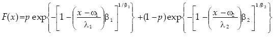
Assuming that first and second populations behave as EV1 and GEV distributions, respectively, equation (1) yields to the six–parameter mixture model of annual floods:

.............................(6)

Where v, α and ω, λ are the location and scale parameters for the first and second population, respectively; β is the shape parameter for the second population.

The corresponding probability density function is

............(7)

Estimation of parameters by maximum likelihood

The likelihood function of n random variables is defined to be the joint density of n random variables and it is a function of the parameters. If X₁ ,X₂,...,X_n is a random sample of a univariate density function, the corresponding likelihood function is (Mood et al., 1974):

.............................................................................(8)

The logarithmic function will be used instead of the likelihood function because it is easier to handle. So, equation (8) is transformed:

.............................................................................(9)

Where L is called the likelihood function, ln is the natural logarithm, θ is the set of parameters to be estimated and f(x,θ) is the EV1–GEV density function, thus

......................(10)

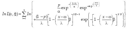
And the corresponding first order partial derivatives of such function with respect to each of the parameters are

.............................................(11)

...........................(12)

..................(13)

.............................(14)

...............(15)

................(16)

The exact solution provided by the system of equations (11)–(16) is not known, so the maximum likelihood estimators of the parameters were obtained by the direct maximization of the log–likelihood function (eq. 10), which is constrained to α>0, λ>0, 0<p<1, and x>0. The suggested procedure is the constrained multivariable Rosenbrock method (Kuester and Mize, 1973).

As it is known, in any of the multivariable constrained non–linear optimization techniques, global optimality is never assured. Therefore, care must be taken in order to avoid a local optimum. It is suggested to start always with values of the location, scale and shape parameters computed by considering the sample divided into two equal parts. If sample is sorted in decreasing order of magnitude, the first set of data is fitted to the univariate GEV distribution (Prescott and Walden, 1980), and the second one to the univariate Gumbel distribution (NERC, 1975). The initial value of the association parameter p will be equal to 0.5.

For the mixed Gumbel and the mixed GEV distributions parameters are estimated following the same optimization procedure.

A region located in Northwestern Mexico, with a total of 35 gauging stations was selected to apply the EV1–GEV distribution to flood frequency analysis. Table 1 shows statistical characteristics of data for each station in the region.

In the area considered in this study, flood outliers correspond to observed rainfall values much higher than the other annual maxima. Such extremely heavy rainfall is due to special meteorological conditions in connection with ENSO events in the Pacific Ocean. In the analyzed area, 62% of the highest annual maximum discharges gauged were generated in an El Niño year and 38% for its counterpart, La Niña.

Results provided by the EV1–GEV distribution were compared with those produced by the mixed Gumbel and mixed GEV distributions. For each station the best one was chosen according to the criterion of minimum standard error of fit (SE), as defined by Kite (1988):

...............................................................(17)

Where g_i,i=1,...n are the h_i,i=1,...n recorded events; are the event magnitudes computed from the probability distribution at probabilities obtained from the sorted ranks of, g_i,i=1,...n,n is the length of record, and q is the number of parameters estimated for the mixed distribution. For the mixed distributions, Gumbel, GEV and EV1–GEV q will be equal to 5, 7 and 6, respectively.

In table 2 is depicted the SE for all mixed distributions along with the best model for the sample of data considered.

The final at–site design events Q (m³/s) for different return periods T(years) in each station are presented in Table 3.

In some sites a comparison is made among different at–site design events (Table 4). For instance, in station Chinipas the computed SE are very similar, however, as return period increases, differences among flood estimates are more significant. A bad selection of the best distribution in the analyzed site can substantially modify the design event and that the hydraulic project might become economically unfeasible or unsafe.

An additional problem is when a short record is used (less than 30 years), because there is an increased risk that the flood estimate will not provide adequate protection of designated uses. One way to reduce the bias or uncertainty in the flood estimate is to use a regional data set with observations from several sites.

This regional technique was not applied in the paper and it just was mentioned to be considered for users in their hydrological analyses.

Conclusions

Floods are often generated by heterogeneous distributions composed of a mixture of two populations. Differences between the populations may be the result of a number of factors such as the El Niño/La Niña oscillations. In the analyzed area 62% of the highest annual maximum discharges (outliers) were generated in an El Niño year. The magnitude of these events is very important and floods can seriously affect people. For this reason, it is necessary to account with an additional mathematical tool that be able to reduce the uncertainty in estimating of design events, which are needed in many water–engineering studies and projects.

In this paper a mixed distribution has been derived by considering different components in an opposite way as usually do. F₁(x) and F₂(x)of equation (1) were the EV1 and the GEV distributions, respectively.

Results shown that there exists a reduction in the standard error of fit when using the EV1–GEV distribution in comparison with the mixed Gumbel or mixed GEV distributions, and just in one out of the 35 analyzed cases, the proposed distribution could not reach convergence in the estimation of parameters process. By contrast, the Mixed GEV distribution had seven failures with the same estimation process.

In 13 sample data the EV1–GEV distribution produced the least standard error of fit (40% of analyzed cases) and in other different cases it was very close to the mixed Gumbel and mixed GEV distributions, However, as it was shown, differences between at–site design events can be significant as return period increases. A bad selection of the best distribution in the analyzed site can substantially modify the design event and also that the hydraulic project might become economically unfeasible or unsafe. Thus, by taking into consideration the mixed flood distributions a more accurate, physically based flood frequency analysis can be obtained and sensible savings in costs of construction of flood protection structures can be expected. This can also improve the setting of flood plain limits and the safety of control structures.

References

Alila Y. and Mtiraoui A. (2002). Implications of Heterogeneous Flood–Frequency Distributions on Traditional Stream–Discharge Prediction Techniques. Hydrological Processes, 16:1065–1084.        [ Links ]

Cavazos T. and Hastenrath S. (1990). Convection and Rainfall Over Mexico and their Modulation by the Southern Oscillation. International Journal of Climatology, 10: 377–386.        [ Links ]

Kite G.W. (1988). Frequency and Risk Analyses in Hydrology. Water Resources Publications, Littleton, Colorado, USA.        [ Links ]

Kuester J.L. and Mize J.H. (1973). Optimization Techniques with FORTRAN. McGraw–Hill.        [ Links ]

Magaña V. and Ambrizzi T. (2005). Dynamics of Subtropical Vertical Motions Over the Americas During El Niño Boreal Winters. Atmósfera, 18(4): 211–233.        [ Links ]

Magaña V., Vázquez J., Pérez J. and Pérez J.B. (2003). Impact of El Niño on Precipitation in Mexico. Geofísica Internacional, 42(3): 313–330.        [ Links ]

Mood A., Graybill F. and Boes D. (1974). Introduction to the Theory of Statistics. Third Ed., McGraw–Hill.        [ Links ]

NERC (1975). Natural Environment Research Council. Flood Studies Report I, Hydrologic Studies. Whitefriars Press Ltd., London, United Kingdom.        [ Links ]

Prescott P. and Walden A. (1980). Maximum Likelihood Estimation of the Parameters of the Generalized Extreme Value Distribution. Biometrika, 67(3): 723–724.        [ Links ]

Raynal J. and Guevara J. (1997). Maximum Likelihood Estimators for the two Populations Gumbel distribution. Hydrological Science and Technology Journal, 13(1–4):47–56.        [ Links ]

Raynal J. and Santillan O. (1986). Maximum Likelihood Estimators of the Parameters of the Mixed GE V Distribution. IX Congreso Nacional de Hidráulica. AMH. Querétaro, Qro., Mex. pp. 79–90. (In Spanish)        [ Links ]

Semblanza del autor

Dr. Carlos Agustín Escalante–Sandoval. Es doctor en ingeniería hidráulica por la Facultad de Ingeniería de la UNAM. Actualmente es profesor titular "C" de tiempo completo definitivo. Ha impartido 85 cursos en el Posgrado de la UNAM; dirigido 38 tesis de maestría y cinco de doctorado. Dentro de su producción académica se encuentran: 30 publicaciones en revistas con arbitraje, 45 en congresos nacionales e internacionales, 3 capítulos en libro, 2 libros como autor y otro como co–editor. Recibió la medalla Gabino Barreda por sus estudios de doctorado, el premio Distinción Universidad Nacional para Jóvenes Académicos en Docencia en Ciencias Exactas 1999 que otorga la UNAM y el Premio Nacional Enzo Levi "Investigación y Docencia en Hidráulica 2002", por parte de la Asociación Mexicana de Hidráulica. Es miembro del Sistema Nacional de Investigadores, Academia Mexicana de Ciencias, Academia de Ingeniería, Colegio de Ingenieros Civiles de México y la Asociación Mexicana de Hidráulica.