Isela Elizabeth Téllez–León**, Francisco Venegas–Martínez*** y Abigail Rodríguez–Nava****
** Escuela Superior de Economía, Instituto Politécnico Nacional. Correo electrónico: tlie_2009@yahoo.com.mx.
*** Escuela Superior de Economía, Instituto Politécnico Nacional. Correo electrónico: fvenegas1111@yahoo.com.mx.
**** Departamento de Producción Económica, Universidad Autónoma Metropolitana–Xochimilco. Correo elecrónico: arnava@correo.xoc.uam.mx.
*Fecha de recepción: 20/03/2011 ]]> Fecha de aceptación: 18/09/2011
ABSTRACT
The aim of this paper is to examine how inflation volatility affects economic growth in a small open economy. To reach this goal, a stochastic macroeconomic model with a financial sector and incomplete financial markets (due to the inclusion of jumps) is developed. It is assumed that the general price level is driven by mixed diffusion–jump process, that is, a Brownian motion governs inflation and a Poisson process guides unexpected and sudden jumps in the price index. The economic growth rate is endogenously determined, in the equilibrium, as a function of parameters of the inflation process.
Keywords: inflation, growth, stochastic models.
Classification JEL: E3, 04, C6.
RESUMEN
El objetivo de esta investigación es examinar cómo la volatilidad en la inflación afecta el crecimiento económico en una economía pequeña y abierta. Para alcanzar este objetivo, se desarrolla un modelo macroeconómico estocástico con un sector financiero y con mercados financieros incompletos (debido a la inclusión de saltos). Se supone que el nivel general de precios es conducido por un proceso estocástico que combina difusiones con saltos, es decir, la inflación es gobernada por un movimiento browniano y los saltos bruscos e inesperados en el índice de precios se rigen por un proceso de Poisson. La tasa de crecimiento económico se determina endógenamente, en el equilibrio, en función de los parámetros del proceso que conduce a la inflación.
Palabras clave: inflación, crecimiento, modelos estocásticos.
]]> Clasificación JEL: E3, 04, C6.
INTRODUCTION
Volatility in the rate of inflation has been one of the distinguishing macroeconomic characteristics, for decades, of many Middle East, Asian, and Latin American economies. While economic literature has provided considerable theoretical advancement in the understanding of the relationship between inflation and growth in the deterministic framework; see, for instance: Hill (2001), Houthakker (1979), Sidrauski (1976), Dornbusch and Frenkel (1973), Phillips (1962), Black (1959), Kaldor (1959), and more recently Loayza y Hnatkovska (2004) y Gonçalves y Salles (2008), it is still missing a stochastic setting that allows modeling properly inflation volatility in order to provide a coherent explanation of the relationship between inflation and growth. We develop a stochastic small open economy model with a financial sector under the assumption of incomplete financial markets. The general price level, which will be endogenously determined, evolves according to a geometric Brownian motion combined with a Poisson process.1 In this case, the Brownian motion models small diffusion movements of the inflation rate and the Poisson process models jumps in the price level. The proposed model considers explicitly the exposure to distinct risks of all the agents. The setting provides tractable closed–forms solutions that make much easier the understanding of the key issues in to explain growth.
In financial and economic literature, the assumption that data follows a log–normal distribution is very common. In particular, it is customary to assume that data follows a geometric Brownian motion. However, there exists strong empirical evidence that most of financial and economic variables of high frequency badly fit a log–normal distribution. One of the main characteristics of these variables is that from time to time they present unexpected jumps, which occur more frequently than it would be expected in a log–normal distribution, even if it a moderate volatility rate is assumed. In macroeconomic data analysis, when a standardized empirical distribution of a variable is compared with a standard normal distribution, it is common to observe that the peak of the empirical distribution is higher than that of the normal case. Since both distributions have the same standard deviation, and hence the same inflection points, the tails of the empirical distribution have to be necessarily fatter in order to compensate its area that must be equal to unity. Thus, a higher peak leads to larger probabilities of small movements and the fatter tails to larger probabilities of extreme values. This distinguishing characteristic is observed in many financial variables, including inflation rates. Mixed diffusion–jump processes provide an alternative to mo–del heavy tails in a richer environment to rationalize price dynamics that cannot be generated by using only the Brownian motion. This fact is not just a sophistication to be included in a macroeconomic equilibrium framework but an important issue to be considered in explaining the relationship between inflation volatility and growth.
This research will develop a general equilibrium stochastic macroeconomic model useful to explain how inflation volatility affects economic growth in a small open economy with a financial sector. Under the assumption of incomplete financial markets, the prices of all available assets (real monetary balance, real bonds and real equity) in the economy will be driven by mixed diffusion–jump processes. Moreover, mixed diffusion–jump stochastic processes will also guide taxes. Finally, we suppose that a Brownian motion governs inflation and a Poisson process guides unexpected and sudden jumps in the price index. The economic growth rate will be endogenously determined in the equilibrium.
This paper extends the basic framework stated in Venegas–Martínez (2009) to assess the impact of the inflation–rate volatility on economic growth. The distinguished characteristics of the current proposal are: 1) the economy is now open; 2) perfect capital mobility; 3) there is a foreign (nominal) bond available in the economy; 4) the representative consumer considers a basket of heterogeneous goods; 5) the probability that the consumes remains alive at time t is driven by the exponential distribution; 6) the mean expected growth is explained in terms of the inflation–rate volatility; 7) and, finally, the mean expected sizes of possible jumps and the intensity parameters of relevant economic variables appear in the mean expected growth rate.
This paper is organized as follows. In the next section, we define the stochastic dynamic of prices and assets. Throughout section III, we state and solve the consumer's decision problem. In section IV, we deal with the firm's decision problem. In section V, we close the model by introducing the government behavior. Through section VI, we determine the stochastic macroeconomic equilibrium. In section VII, we determined, endogenously, the expected growth rate of output. Finally, we present conclusions, acknowledge limitations, and make suggestions for further research. One appendix contains a useful theoretical result for the development of the proposed model.
I. EMPIRICAL STYLIZED FACTS
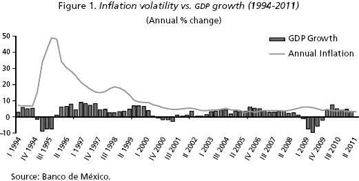
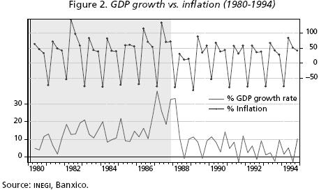
]]> In this section, we revise some stylized facts. The major episodes of inflation volatility observed in Mexico are: mid–1995, 1999, 2001 and 2009, which lead to a reduction in the growth rate of GDP. It is important to point out that in some periods there was even a decrease of output, as seen during some years between 1980 and 1994; see Figures 1 and 2.
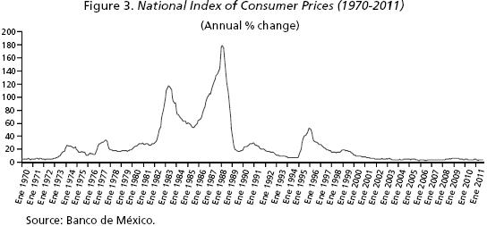
The volatility of inflation may be due to the existence of sharp fluctuations in supply and demand in raw materials and agricultural products or fuels, which are fundamental to many aspects of daily economic activities. Moreover, the unstable behavior of prices could have negative effects in saving and investment, creating inefficiencies in the market. Notice the volatile behavior of the National Index of Consumer Prices in Mexico during some periods in 19702011, as shown in Figure 3.
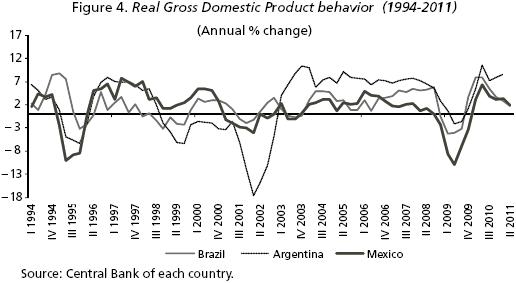
The stylized fact sated above, namely that high volatility of inflation leading to lower growth is not only observed in Mexico, but also in other small open economies in Latin American (for instance, Mexico, Brazil, and Argentina). The higher fluctuations in inflation have negative effects forbusinesses and consumers, which could result in reducing growth rates, as it can be see in Figure 4.
]]>
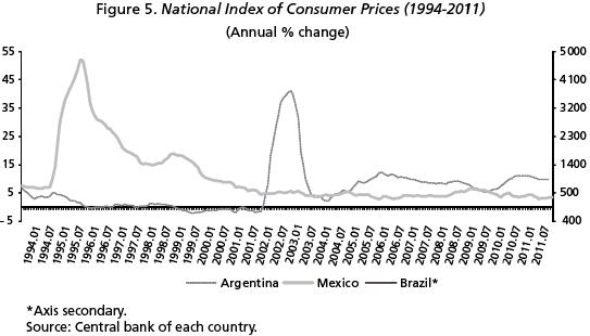
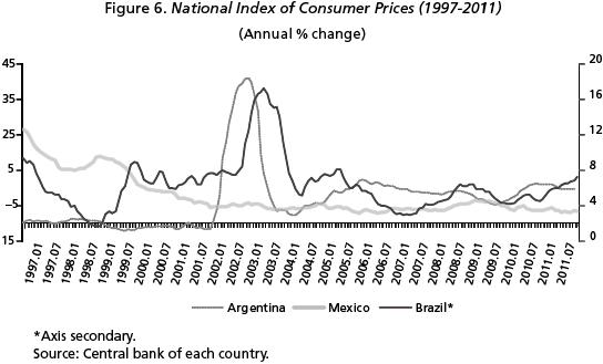
When the inflation rate is volatile, prices are unpredictable for consumer and businesses to plan consumption and production, respectively, in the long term. Finally, in Figures 5 and 6 it is shown the dynamics of National Index of Consumer Prices for some small open economies during different periods of time.
II. PRICES AND REAL SECURITIES
Let us consider a small open economy with a single (representative) infinitely lived consumer in a world with a single perishable consumption good. We also contemplate in this economy a single (representative) firm that uses available capital to produce domestic output. And in this section, we establish the dynamics of asset prices to treat the consumer's problem.
We assume that the good is freely traded, and its domestic price level, Pt, is determined by the purchasing power parity condition, namely Pt =Pt*Et where Pt* is the foreign–currency price of the good in the rest of world, and Et is the nominal exchange rate. Since the consumer is price taker in all of his trading activities with the rest of the world, we may suppose, for the sake of simplicity that Pt* remains constant over time. We also assume that the price level, Pt, and consequently the exchange rate, Et, is driven by a mixed diffusion–jump process according to:
]]>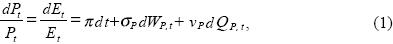
Where the drift (or physical trend) π is the mean expected rate of inflation (or mean expected rate of depreciation) conditional on no jumps, σP is the instantaneous standard deviation or volatility of expected inflation, and 1 + vP is the mean expected size of possible jumps in the general price level. Here, WP,t stands for a standardized Wiener process, that is, WP,t is a temporally independent normally distributed random variable with E [dWP,t] = 0 y Var[dWP,tJ = dt. The initial price level P0= E0 is supposed to be known, positive, and deterministic. We also assume that jumps in the price level follows a Poisson process, QP,t , with intensity parameter λP , in such way that:

whereas2:
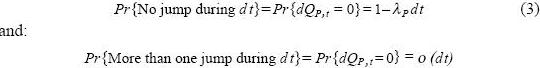
Henee, E [dQp,t]=Var[d Qp, t] = λp dt. The initial number of jumps is supposed to be zero, that is, QP,0= 0. Throughout the paper, we will assume that Wp,t and QP,t are uneorrelated processes. The trend π, the volatility σP, the mean jump amplitude vp, and the probability of a jump in the price level Pr{dQP,t=1} are to be all endogenously determined.
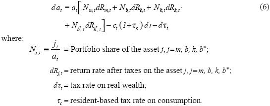
The representative consumer possesses four different assets: domestie (nominal) money, Mt; domestic (nominal) government bonds, Bt; equity claims, kt; and foreign (nominal) bonds, Bt*. Therefore, the individual's real wealth, at, in terms of the consumption good as numeraire is given by:

where mt= MtlPt stands for real monetary balances, bt= Bt Pt represents the holding of domestic bond in real terms, and:

We next determine the asset returns. We suppose that the nominal rate of return on money and bonds are zero and i, respectively. The stochastic rate of return of holding real monetary balances at time t, dRm,t, is simply the percentage change of the price of money in terms of goods. A straightforward application of Itó's lemma to the percentage change of real balances, taking (1) as the underlying process, leads to (see Appendix):
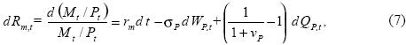
where rm = – π + σ2P. The stochastic return of holding bonds is similarly obtained
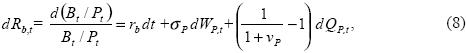
where rb = i(l – τy) – π + σ2P, and τy is the tax rate on interest income. It is worth–while to observe that both the stochastic rate of return on domestic money and bonds are affected by the volatility and jumps in the general price level. The stochastic rate of return on equities after taxes will be denoted, for the time being, as:

where Wk,t is a Wiener process and Qk,t is a Poisson process with intensity parameter λk. The process dRk,t will be endogenously determined in the macroeconomic equilibrium. Finally, the stochastic rate of return on foreign bonds is deterministic and given by:
db*t = b*tdRb*, t = bt*rb, dt.
]]> The only remaining issue is how taxes are paid, we suppose that the consumer pays a tax on wealth as follows:
where  is the mean expected tax rate on real wealth. As before, Wtand Qτ, t are a Wiener and a Poisson processes, respectively. The trend , as well as the diffusion and jump components στdWτ,t y vτ, t dQτ, t are to be endogenously determined. All of the processes Qp,t, Qk,t and Qτ, t are supposed to be mutually uncorrelated.
III. CONSUMER'S DECISION PROBLEM
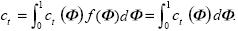
Consider a small open economy populated by agents with identical preferences Suppose that the representative consumer derives utility from a generic consumption good and from the liquidity services of real balances. It is also assumed the the consumption of heterogeneous goods, ct (Φ), indexed by Φ  [0,1], have a uniform density in [0,1], that is:
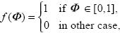
in such way the consumption of the aggregate basket is given by:
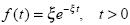
It is also assumed that the density function that consumes remains alive at time t is exponential with parameter ξ that is:
]]>
We assume that the expected utility is of the Von Neumann–Morgenstern type. Specifically, the total discounted expected utility at time t = 0, V0, of the competitive consumer has the following separable form:
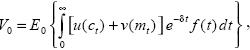
where E0 is the conditional expectation upon all available information at time t = 0, and δ is the agent's subjective discount rate. In particular, we choose u(ct) = θlog(ct), and v(mt) = (1 – θ) log(mt), 0 < θ < 1, in order to generate closed–form solutions that makes the analysis tractable. Under this utility index the consumer becomes a risk–averse agent. Thus, the objective of the consumer is to choose, at each instant, the portfolio shares and the consumption amount that maximize his utility index. Moreover, it is important to point out that the main results or conclusions may not be valid under other specifications of the utility fimction. If more general functional forms are considered, it is possible than closeform solutions are not obtained, and in some cases even only numerical approximate solutions can be found. However, we may anticipate that results do vary when using other utility functions; for instance, when using the negative exponential utility function or the hyperbolic utility index, which is out of the reach of objectives' paper.
After substituting expressions (7) – (10) in the stochastic equation of wealth accumulation (6), we get:
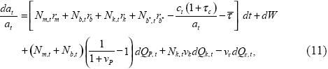
where the diffusion component satisfies:

The necessary conditions for an interior solution of maximizing V0 subject to (11) and to the normalizing constraint:
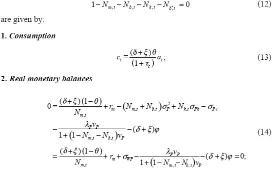
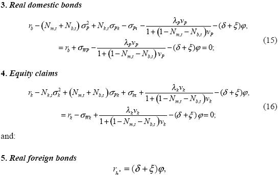
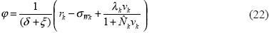
where φ is the Lagrange multiplier associated with the constraint (12), Cov (dW,σP WP,t) = σWPdt, and Cov (dW, σk Wk,t) = σWkdt. Equation (13) simply expresses that consumption is proportional to real wealth. After subtracting (14) from (15), we readily find that the optimal portfolio share on real monetary balances is given by:
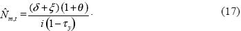
Hence, the portfolio share of real money balances varies inversely with the after–tax nominal interest rate. Moreover, after subtracting (15) from (16), we get:
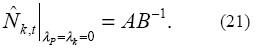
Clearly, equation (18) is cubic with real coefficients, and hence it has at least one real solution,3 which will be denoted by Ñk,t. Observe that we have not imposed constraints on the portfolio shares to be strictly positive and less than unity, and hence short sales are permitted at any time. In particular, if we assume that λP and λk are zero, then C = D = 0, and there is a unique solution (cf. Turnovsky, 1993):
Observe now that from (16), we can obtain the value of the Lagrange multiplier:
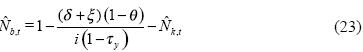
Finally, the optimal portfolio is completely determined with  b,t, which is residually obtained from (l2) as:
Since optimal portfolio shares remain constant over time, in what follows we will leave out the time sub index, and we will simply write: m, b, and k. Finally, notice that the first–order conditions can be rewritten in terms of marginal utility as:

Moreover, in virtue of (14), (23) and (18), we may re write (25) as follows:
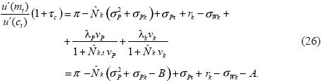
The above equation equals the marginal utility of holding real balances, standardized by the marginal utility marginal of consumption, with the marginal cost of holding real balances. This condition shows explicitly how the opportunity cost of money is affected by uncertainty, i.e., by small diffusive changes in inflation and by chronic extreme movements in the price level. Finally, observe that logarithmic utility implies that the optimal values of j , j = m, b, k, depend only on in the parameters that determine preferences and stochastic characteristics of the economy. In other words, the consumer's attitude to risk is independent of the real wealth level, i.e., the resultant real wealth level at any instant has no effects on the portfolio decisions.
IV. FIRM'S DECISION PROBLEM
In microeconomic theory is common to assume that firms conduct research and development in search of technological change. Due to the constant search for greater profits, companies try to get maximum benefit in the technologies adopted. One such advantage is access to more efficient production conditions and distribution, via the technological change. It is here the main motivation for a firm to invest resources in research and technological development. In this context, consider a firm whose production, y, depends on a capital asset, kt. It is assumed that small changes in technology that are seen every day are driven by a diffusion process (Brownian motion or Wiener process), and technological innovations (technological leaps) that occasionally occur are modeled with a Poisson process. The technology used by the firm can be owned or acquired from other companies, private or public.
Suppose that in the domestic economy there is only one firm that uses all available capital to produce domestic output. Available capital is the domestically produced output that is not consumed, purchased by the government, or exported. The rate of return on equity will be determined in terms of the production level and the dividends policy. We assume that production is driven by the following stochastic technology:
]]>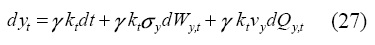
where γ represents the mean expected marginal product of capital. Here, as in the consumer case, Wy,t is a Wiener process and Qy,t is a Poisson process with the standard characteristics. Processes σy,tdWy,t and vydQy,t are supposed to be exoge–nous. In general terms, the return on equity can be defined as:
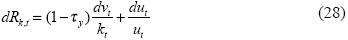
where vt is flow of dividend payments and ut is the equity price on real terms. We suppose that capital gains are no taxed.4 Notice that the return on capital has two components: the dividends paid by each share and the gains or losses of capital as a result of the difference in prices. Let us examine each component separately. In order to determine the percentage change of ut, dut / ut, it is necessary to analyze all the variables determining possible capital gains: number of shares, production and investment. For the sake of simplicity, we will assume that number of shares, at any time, t, remains constant, say equals to N, then it follows that Nut=kt. Therefore:

On the other hand, production after corporate income tax can be used either to pay out dividends, dvt, or to finance investment, dkt, i.e., acquisition of new capital. Hence, the change in output after taxes is given by:

where τP is the tax on corporative income. By combining equations (29) and (30), we get:
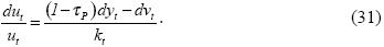
Substituting the above expression in (28), we get:
]]>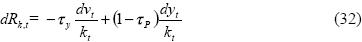
On the other hand, the dividend policy of a firm is a plan for the distribution of payments of dividends to shareholders. The dividend policy should take into account two basic aspects: maximize the benefit of the owners of the company and provide sufficient funding for the company, including research and development. A cash dividend per share of the company indicates the percentage per dollar distributed to shareholders. One of the drawbacks of this policy is that if company profits decline, or if a loss occurs in a given period, dividends may be low or even zero, pushing the plan previously established. A regular dividend policy is based on paying a fixed dividend in each period. This policy gives share–holders confidence, indicating that the company performs well, thus reducing uncertainty. There is also the possibility of payment of stock dividends, a stock dividend is the payment of dividends in shares to existing owners and the companies often resort to such dividend as a form of replacement or addition of dividends. The proposed modeling assumes that the firm pays dividends at a constant fraction aof the after–tax corporate income. That is, dividends have the following form:

After substituting this expression in (32), we obtain the stochastic process governing the return on capital in terms of the technology process as:
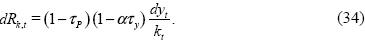
It is important to point out that in the above equation its stochastic behavior is due to dyt /kt, since the rest of the variables in (34) are deterministic. Finally, equation (9) is fully determined by:

Thus, the rate of return on equity depends upon the marginal product of capital. Similarly, the stochastic components dRk,t depends on the productivity shocks from changes in y an from the exogenous behavior of dWy,t and dQy,t.
V. GOVERNMENT BEHAVIOR
]]> In order to close the model, we describe the government actions as well as the public policy. The public sector generates no utility for the consumer, has the monopoly of printing money, and issues debt to finance public expenditures. The government budget constraint in real terms has the form:
where dgt is the change of public expenditures; dτ1, t is the change in taxes paid by the consumer; dτ2, t is the change of taxes paid by the firm. We next summarize the government policy variables, namely: public expenditures, money supply, and public debt.
In our proposed framework, government expenditure is driven by the following stochastic process:

where  is the mean expected rate of fiscal expenditure. As before, Wg,t is a Wiener process and Qg,t is a Poisson process. Notice that government expenditures are defined as a fraction of production. Money supply is a driven by a mixed diffusion–jump process as follows:

where µ is mean expected rate of monetary expansion, dWM,t is the diffusion component, and dQM,t is the jump component. Public debt is issued in such a way that the bond–money ratio remains constant over time, that is:
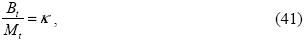
where κ is a known constant. Hence, it follows, immediately, that:
]]>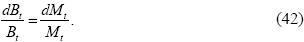
Therefore, in open market operations, the percentage change of issued debt is equal to the percentage change of shorts in money supply, or equivalently, the percentage change in money supply is equal to the percentage change of the debt liquidation.
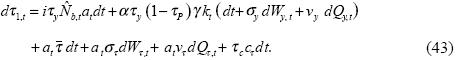
The changes of total taxes in real terms, dτ1,t and dτ2,t, paid by the consumers and firms, respectively, are now described. Recall that the remaining taxes τy, τP and τc, are exogenous in our model. Hence, the total tax collected by the government from consumers is given by:
In the firm's case, there is only a tax on corporate income, that is:

VI. EQUILIBRIUM CONDITIONS
In this section, we find the macroeconomic equilibrium and the stochastic rate of capital accumulation in the economy, dkt/kt, we use the national income identity:

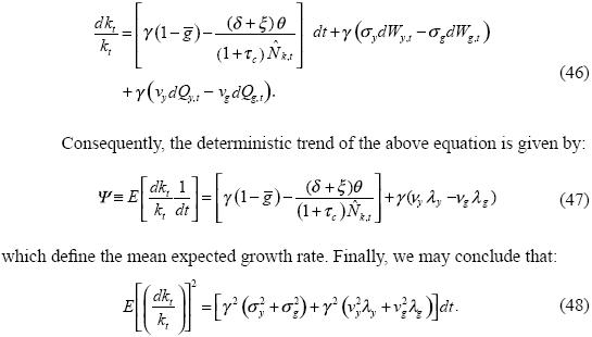
In other words, the variance of capital accumulations depends upon the variances of both the diffusion and jump components. This result will be used to determine the overall macroeconomic equilibrium. Once we have determined the agent's optimal decisions, the firm behavior, the government actions, and the policy variables, it remains to obtain the macroeconomic equilibrium. By using the fact that real balances and government bonds in real terms are linked with movements in the price level, we may determine endogenously the inflation rate. Notice now that we can rewrite the price level as:
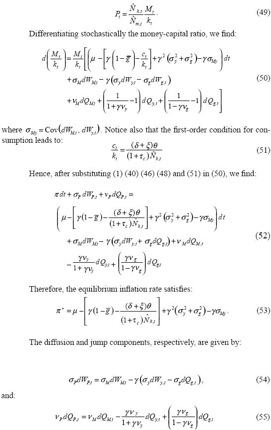
Equations (53)–(55) determine endogenously the rate of inflation consistent with constant optimal portfolio shares. We observe in (53) that the equilibrium inflation is positively affected by the rate of monetary expansion, negatively affected by the mean expected growth rate of capital, and positively affected by the variances of fiscal and production diffusion and jumps shocks. On the other hand, equations (54) and (55) determining endogenously the diffusion and jump stochastic components of the equilibrium inflation rate. It is important to point out that these components are functions that depends upon the exogenous stochastic behavior of the rate of money supply, production technology and government expenditures.
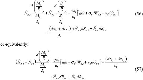
In order to determine the endogenous adjustment in fiscal policy, we use the fact that the government budget constraint must be satisfied. First, by substituting the equations of government expenditures (39), money supply (40), and debt policy (41), in (38) we find:
On the other hand, by applying Itó's lemma to obtain the stochastic differential d (Mt / Pt) with (1) and (40) as the underlying stochastic processes, we get:
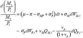
After substituting the above expression along with those for the taxes dτ1,t and dτ2,t in (57), we have that the deterministic and stochastic components of the equilibrium tax adjustment are given by:
]]>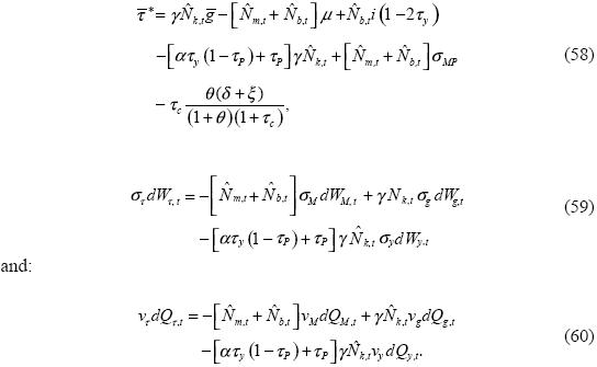
Equation (58) describes the endogenous adjustment in the deterministic component, while equation (59) summarizes the diffusion part as a functions of random fluctuations in the rate of monetary expansion, σM dWM,t , government expenditures, σgdWg,t, and the real sector, σydWy,t. The jump component given by (60) is a function of the stochastic jump components of the rate of monetary expansion, the production technology and the public expenditures.
VII. MEAN EXPECTED GROWTH RATE
Finally, to determine the equilibrium rates of return of the real balances and bonds in real terms, we substitute the above expressions in (7) y (8), respectively, so the rate of return of holding money is given by:
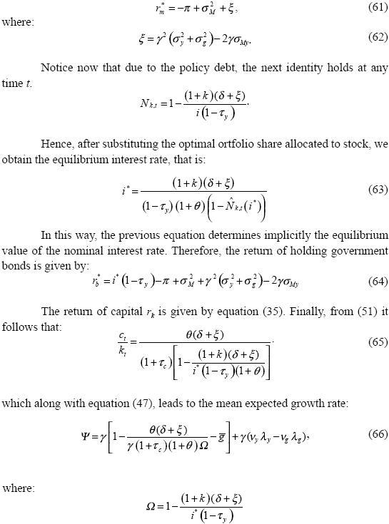
Notice that economic growth is primarily driven by improvements in the growth rate of capital, which involves producing more goods maintaining without change the other inputs. Observe now that in virtue of rb* = i* (1 –τy) – π* + σ2P, we get:
Equations (66) and (67) offer an explicit relationship between inflation volatility and output growth. In such a relationship, clearly, an increase in inflation volatility, σP, in (67), leads to a reduction in the economic growth rate Ψ, in (66). Indeed, an increase in σP decreases i*, which in turn reduces Ω, which appears in the denominator of first term of (66). Hence, the total effect of the whole first term is negative. Thus, the proposed model provides a negative correlation between volatility in the general price level and the growth rate of output in a small open economy with a financial sector. In this way, our approach has acquainted with an endogenous growth model consistent with stylized facts that highlight the relationship between nominal volatility and growth.
]]> CONCLUSIONS
Monetary authorities often motivate their concerns about inflation by claiming that price level stability contributes to economic growth. Consistently, our theoretical approach has shown that in the long run countries having experienced high inflation volatility also tend to feature dismal growth performances. We have developed a macroeconomic equilibrium model in a richer stochastic environment is useful to examine how inflation volatility affects economic growth. The exogenous variables include the economic policy parameters: rate of monetary expansion, µ; public expenditures, ; debt policy, k; and the tax rates τy, τc and τP. Similarly, the exogenous stochastic processes are: money growth rate, dWM,t, public expenditures, dWg,t, and production, dWy,t. The rest of the stochastic processes are endogenous and can be expressed as functions of exogenous shocks. The economic growth rate was endogenously determined in the equilibrium, as a function of parameters of the process driving inflation, which have an important role in the design of economic policy.
It is also important to point out that in the proposed theoretical framework, as in the second term in equation (66), the mean expected marginal product of capital, γ the expected size of a technological jump affect, vy, and the probability that such a jumps occurs, λy, all of them impact positively the growth rate Ψ, since economic growth is primarily driven by improvements in capital productivity, which leads to producing more goods and services with the same inputs of labor, energy and materials.
Needless to say, more research is required to assess the effects on economic welfare and indirect utility. An important question is if countries featuring high inflation volatility tend to have underdeveloped financial markets and dismal growth performances, of course this issue will be treated in future investigations. It is also important to point out that the main results may not be valid under other specifications of the utility function, and future research will be devoted to more general functional forms of the satisfaction index.
APPENDIX: ITÔ'S LEMMA ON THE RATIO OF TWO PROCESSES
REFERENCES
Black, John (1959), "Inflation and Long–Run Growth", Económica, Vol. 26, No. 102, pp. 145–153. [ Links ]
]]>Dornbusch, Rudinger and Jacob. A. Frenkel (1973), "Inflation and Growth: Alternative Approaches", Journal of Money, Credit and Banking, Vol. 5, No. 1, pp. 141–156. [ Links ]
Gihman, Iosif Ilich and Anatolií Vladimirovich Skorohod (1972), Stochastic Differential Equations, Springer–Verlag, Berlin. [ Links ]
Giuliano, Paola and Stephen. J. Turnovsky (2003), "Intertemporal Substitution, Risk Aversion, and Economic Performance in a Stochastically Growing Open Economy", Journal of International Money and Finance, Vol. 22, No. 4, pp. 529–556. [ Links ]
Gonçalves, Eduardo S. and João M. Salles (2008), "Inflation Targeting in Emerging Economies: What Do the Data Say?", Journal of DevelopmentEconomics, Vol. 85, No. 1–2, pp. 312–318. [ Links ]
Grinols, Earl L., and Stephen S. Turnovsky (1993), "Risk, the Financial Market, and Macroeconomic Equilibrium", Journal of Economic Dynamics and Control, Vol. 17, No. 1–2, pp. 1–36. [ Links ]
]]>Hill, Robert J. (2001), "Measuring Inflation and Growth Using Spanning Trees", International Economic Review, Vol. 42, No. 1, pp. 167–185. [ Links ]
Houthakker, Hendrik S. (1979), "Growth and Inflation: Analysis by Industry", Brookings Papers on Economic Activity, Vol. 1979, No. 1, pp. 241–256. [ Links ]
Kaldor, Nicholas (1959), "Economic Growth and the Problem of Inflation", Economica, Vol. 26, No. 104, pp. 287–298. [ Links ]
Loayza, Norman and Viktoria V. Hnatkovska (2004), Volatility and Growth. World Bank Policy Research, Working Paper, No. 3184 [ Links ]
Phillips, Alban William Housego (1962), "Employment, Inflation and Growth", Economica, Vol. 29, No. 113, pp. 1–16. [ Links ]
Sidrauski, Miguel (1976), "Inflation and Economic Growth", The Journal of Political Economy, Vol. 75, No. 6, pp. 796–810. [ Links ]
Turnovsky, Stephen J. (1993), "Macroeconomic Policies, Growth, and Welfare in a Stochastic Economy", Journal of Economic Dynamics and Control, Vol. 34, No. 4, pp. 953–981. [ Links ]
Turnovsky, Stephen J.(1999), "On the Role of Government in a Stochastically Growing Open Economy", Journal of Economic Dynamics and Control, Vol. 23, No. 5, pp. 873–908. [ Links ]
Venegas–Martínez, Francisco (2009), "Un modelo estocástico de equilibrio macroeconómico: acumulación de capital, inflación y política fiscal", Investigación Económica, Vol. 68, No. 268, pp. 69–114. [ Links ]
* The authors wish to acknowledge the valuable and helpful comments and suggestions from anonymous referees, which had greater repercussions in improving this research.
]]> 1 There are many works in the economic literature that use diffusion or mixed jump–diffusion proces, we mention, for instance: Grinols and Turnovsky (1993), Turnovsky (1993), and Giuliano and Turnovsky (2003). 2 As customary, o(h) means that o(h)/ h 0 as h0.
3 Indeed, non real roots occur in conjugate pairs.
4 We assume, as in the Mexican case, that there is not a tax on capital gains.
5 For the proofs, we refer the reader to Gihman and Skorohod (1972).
]]>