
FRANCISCO ESTRADA
Centro de Ciencias de la Atmósfera, Universidad Nacional Autónoma de México, Circuito de la Investigación Científica s/n, Ciudad Universitaria, 04510 México, D.F. Institute for Environmental Studies, VU University Amsterdam, De Boelalaan 1087, 1081 HV Amsterdam, The Netherlands Corresponding author: feporrua@atmosfera.unam.mx
VÍCTOR M. GUERRERO
Departamento de Estadística, Instituto Tecnológico Autónomo de México (ITAM), Río Hondo 1, Col. Progreso Tizapán, 01080 México, D.F.
Received March 4, 2014; accepted September 3, 2014
]]>RESUMEN
Este trabajo propone una metodología para elaborar escenarios de cambio climático a escala local. Se usan modelos multivariados de series de tiempo para obtener pronósticos restringidos y se avanza en la literatura sobre métodos estadísticos de reducción de escala en varios aspectos. Así se logra: i) una mejor representación del clima a escala local; ii) evitar la posible ocurrencia de relaciones espurias entre variables de gran y pequeña escalas; iii) una representación apropiada de la variabilidad de las series en los escenarios de cambio climático, y iv) evaluar la compatibilidad y combinar la información de variables climáticas con las derivadas de los modelos de clima. La metodología propuesta es útil para integrar escenarios sobre la evolución de los factores de pequeña escala que influyen en el clima local. De esta forma, al escoger distintas evoluciones que representen, por ejemplo, distintas políticas públicas sobre uso del suelo o control de contaminantes, la metodología ofrece una manera de evaluar la conveniencia de dichas políticas en términos de sus efectos para amplificar o atenuar los impactos del cambio climático.
ABSTRACT
This paper proposes a new methodology for generating climate change scenarios at the local scale based on multivariate time series models and restricted forecasting techniques. This methodology offers considerable advantages over the current statistical downscaling techniques such as: (i) it provides a better representation of climate at the local scale; (ii) it avoids the occurrence of spurious relationships between the large and local scale variables; (iii) it offers a more appropriate representation ofvariability in the downscaled scenarios; and (iv) it allows for compatibility assessment and combination of the information contained in both observed and simulated climate variables. Furthermore, this methodology is useful for integrating scenarios of local scale factors that affect local climate. As such, the convenience of different public policies regarding, for example, land use change or atmospheric pollution control can be evaluated in terms of their effects for amplifying or reducing climate change impacts.
Keywords: Compatibility testing, downscaling techniques, multiple time series models, restricted forecasts, statistical model validation, climate change.
1. Introduction
Coupled ocean-atmosphere general circulation models (AOGCM) provide the most complete representation of the climate system to date and occupy the highest position in the hierarchy of climate models. These models are used to study and simulate climate at the global and regional scales as well as for generating forecasts and projections for a wide range of time-horizons (IPCC, 2007). During the past two decades, these models have seen great improvements with respect to the number and complexity of the climate system processes that they simulate, their capacity to adequately reproduce the observed regional and global climate, as well as the temporal and spatial resolution they can provide.
]]> However, the spatial resolution required for many applications is frequently higher than what even the most advanced physical climate models can currently offer. To address such needs, downscaling techniques have been developed and are commonly used for evaluating the potential impacts of climate change as well as the convenience of adopting possible adaptation options. There are two main approaches for implementing downscaling: (1) dynamic methods in which the finer-scale regionalization is produced by regional (limited area) physical climate models; and (2) statistical methods in which the downscaling is obtained by means of linear/nonlinear regression, canonical correlation and neural networks, among other statistical models (Wilby et al, 2004). Down-scaling can be defined as "the process of making the link between the state of some variable representing a large space and the state of some variable representing a much smaller space" (Benestad et al., 2008). The following equation provides a central framework for downscaling methods
where local climate (y) is a function of local physiographic features (l), large-scale factors (X) and global climate (G). Downscaling methods, whether dynamic or statistical, have the objective of linking the local climate to these three factors (von Storch et al., 2000; Wilby et al., 2004; Benestad et al., 2008).
Statistical downscaling assumes the existence of a strong, underlying physical mechanism supporting the existence of a relationship between the large- and local-scale variables. Some of the most important advantages of statistical downscaling over dynamic methods that have been discussed in the literature (e.g., Wilby et al, 2004; Benestad et al., 2008) are: (i) it is computationally cheap and thus it allows to create large sets of local scenarios based on different combinations of emissions scenarios and climate models. This characteristic makes statistical downscaling particularly convenient for exploring climate change uncertainty at the local level; (ii) it can be tailored to meet the user's specific demands in terms of climate variables and particular locations; (iii) it can be used to further downscale the output of regional climate models.
According to Benestad et al. (2008), Wilby et al. (2004), von Storch et al. (1993, 2000), Wilby and Wigley (1997, 2000), and Giorgi et al. (2001), some of the assumptions that need to be satisfied in order to assure the theoretical validity of the statistical downscaling are:
i. The existence of a physical mechanism supporting the relationship between local and large scale variables.
ii. That the predictors used for building the statistical model are adequately reproduced (realistically simulated) by the climate model at the same spatial and temporal scales - choosing predictors is frequently determined by a trade-off between the predictors' relevance for explaining the variable of interest and the climate models' skill to simulate them.
iii. That the relationship between predictors and predictand remains stable over time, i.e. the relationship between the large and local scale variables must be stationary. Some of the factors that can potentially generate nonstationarities in this relationship are changes in local land cover and land use, caused for example by deforestation and urbanization. Another possible cause for nonstationarities is that changes in global climate have effects over the regional and local climate in ways that are not captured by climate models.
In general, the effects of local factors and global changes in climate are assumed to be constant, leading to the following simplified version of Eq. (1.1)

iv. The set of predictor variables must fully represent the climate change signal and both the predictand and predictor should respond in a similar way to a given perturbation (e.g., changes in the atmospheric concentrations of greenhouse gases) in order to be useful for downscaling purposes.
v. The predictors used for projecting the local future climate should not be outside the range of the climatology used for calibrating the statistical downscaling model.
As discussed in Estrada et al. (2013a), the assumptions commonly required in the literature for the downscaling model to be valid are not necessarily related to those that would be required for the underlying statistical model to be adequate. Statistical downscaling tends to be addressed as a problem of minimizing some error measure or maximizing some goodness of fit measure. For example, Benestad et al. (2008) refers to the model calibration as the part of the downscaling process where different weights are applied to the different predictor series in order to achieve the best fit or the optimal fit. Estrada et al. (2013a) discuss in detail the drawbacks and implications of this approach and propose an alternative methodology based on statistically adequate models for constructing local climate change scenarios. They also stress that when statistical downscaling is applied, a probabilistic model is being proposed. As such, for the statistical downscaling to be valid the empirical validity of the assumptions of the underlying probabilistic model needs to be evaluated. This paper extends Estrada et al. (2013a) to multivariate time series modeling in order to produce a novel approach for downscaling climate change scenarios based on VAR (vector auto-regressive) models and restricted forecasting techniques.
This paper is structured as follows. Section 2 briefly reviews the VAR methodology and the restricted forecast technique applied to these models. The advantages of this approach over other currently available statistical methods for downscaling are discussed. Section 3 presents a description of Mexico City in terms of its microclimates, topography and levels of urbanization. It also discusses the length and quality of climate records that are available for this city. Section 4 shows that the effects of local factors (urbanization and atmospheric pollution) over the local climate can have large impacts on the resulting downscaled climate change projections. Contrary to what is assumed by automated down-scaling toolkits and a large part of the climate change impacts literature, downscaling is still an unsolved issue plagued with methodological, conceptual and application problems. This section argues that given the large impact that local forcing factors can have on the local climate, creating future scenarios for these factors is as important as for factors determining the global and regional changes in climate. If the evolution of local forcing factors is neglected or extrapolated using current trends, as is currently done in most downscaling applications, local projections may not be physically consistent. It is emphasized that downscaled scenarios should be interpreted as conditional on, for example, the selection of the emissions scenario and global climate model, the parameter stability in the statistical model and the assumed evolution of local factors, among others. Section 5 presents the conclusions.
2. Statistical methodology
2.1 VAR models
A VAR model is a generalization of an autoregressive model useful to represent multiple time series with no need to impose restrictions based on the theory behind the phenomenon under study. In this sense, VAR models are free oftheory (Sims, 1980; Greene, 2002; Zivot and Wang, 2005). They are preferable to univariate models because they offer the possibility to understand the dynamic structure among the series and to improve forecasting accuracy (Peña et al, 2001). VAR models can be interpreted as: (i) a reduced form of a theoretical structural model or a transfer function; (ii) an approximation to a general vector autoregressive and moving average (VARMA) model (Lütkepohl, 2005); and (iii) a simple representation that captures the empirical regularities of an observed multivariate time series. A finite order VAR model can be expressed as

where the k-variate column vector Zt = (Zu, Zkt)' represents a multiple time series and the apostrophe indicates transposition; n (B) = Ik - ΠlB -... - ΠPBP is a matrix polynomial of order P < ∞; Ik is the identity matrix of order k; n is a constant coefficient matrix of dimension k x k, with elements πi,j,f for i, f = 1, k and j = 1, P; the vector μ = (μi...μk)' contains some reference levels for the series; and {at} denotes a sequence of independent and identically distributed random vectors, with distribution a ~ Nk(0k, Σa), where cov(ait, ajt) for all i ± j and  = var(ait) for i = 1, k and t = 1, N.

with Dt a vector of deterministic variables.
2.2 Restricted forecasts
Restricted forecasts generated with time series models are useful to incorporate additional information to that provided by a historical series. In principle, it is convenient to see how the forecasts are generated exclusively on the basis of a historical record of the series. For simplicity of exposition, we consider that the true parameter values are known. Let Z = (Z1,...,ZN) be the vector of historical data and ZF = (Z N+1,...,ZN-H) be the vector of future values to be forecasted, with origin at Nfor the time horizon H ≥ 1. The optimal forecast, in minimum mean square error (MMSE) sense, is given by the conditional expectation
and its forecast error is

The forecast error vector is ZF - E(ZF|Z) = ΨaF, with Ψ a lower block diagonal matrix of size kH x kH, with Ik on the diagonal, Ψ1 on the first sub-diagonal, Ψ2 on the second sub-diagonal and so on. The matrices Ψi , for j = 1, 2, ... , are calculated from the following recursion (see Wei, 1990, p. 364) which is valid both for stationary and nonstationary series
We can improve on the VAR forecasts if we take into account extra-model information by means of restricted forecasting, as shown by Guerrero (2007) and Guerrero et al. (2008). To see this, let Y = YtJ' be a vector of future values or forecasts of a new variable, coming from an external source to that used for building the VAR model. Such a vector is related to the vector of future values of Z by means of the stochastic linear combination Y = CZF + u where (u1,...uM)' is a random vector with E(u|Z) = 0, i.e., the restrictions imposed by Y on Z are conditionally unbiased, but uncertain, since they are associated to a variance-covariance matrix var(u|Z) = Σ u; of course, when Yu = 0 the restrictions become certain. Besides, C is a known M x kH matrix of rank M < H, whose rows contain the M linear combinations defining the restrictions.
The optimal restricted forecast of ZF and its MMSE matrix are given by

and

respectively, with 
 . Additionally, we can test for both total and partial compatibility of the two different sources of information involved. When the test statistic does not produce a significant value we say that the two sources are compatible, the opposite occurs when the test is significant and a possible explanation for this is that a structural change is expected to occur during the forecast horizon, as considered by Guerrero et al. (2013). The calculated test statistics for total and partial compatibility are, respectively,

to be compared with values of a x M distribution, and
As it is shown below, VAR models together with restricted forecasting produce a new way of carrying out statistical downscaling. With this new approach to estimate changes in local climate, there is no need of estimating the relationship between large scale and local variables. Moreover, we can also model the interaction among neighbor series, in such a way as to get a better representation of weather at the local level.
3. Building a VAR model for Mexico City
3.1 Description of the place of study
Mexico City (MC) has an extension of 1485 km2 and it is located in an endorreic basin surrounded by mountains (CONAPO, 2002). Its average elevation is 2240 masl, with its lowest point in the northeast and highest towards the southeast. These features produce a tropical climate, tempered by altitude (Jauregui, 2000). Furthermore, the central-north part of MC that covers 45% of its area has mostly urban land use, while the remaining 55% located in the south-southwest has basically rural land use.
There is a great deal of anthropogenic and local natural factors that modulate the large-scale climatic factors. Among the natural factors we can find topography, elevation, vegetal coverage and the presence of water bodies; among the most important anthropogenic factors we can mention density and building type, atmospheric pollution and land use changes (Estrada et al, 2009). Several works on urban climatology (e.g., Jones et al, 1990; Jauregui, 1991; Ishi et al, 1991) have shown that urbanization and deforestation have an important effect on the city climate, making it warmer and dryer. In spite of the small geographical space covered by MC, local factors such as its complex topography and level of urbanization make it a place with a highly heterogeneous climate. Estrada et al. (2009) applied multivariate statistical techniques to analyze the data produced by 37 meteorological stations of the Servicio Meteorológico Nacional (National Meteorological Service) and found two large climatic regions in MC, as well as four sub-regions. The two large regions are basically defined by their topography - they divide the city in low altitude (northeast-center) and high altitude areas (southwest, where the mountains begin) - while the four sub-regions are defined not only by the effect of geographic factors but also by that of anthropogenic ones.
Sub-region 1 (S1) is located in the eastmost and lowest part of the city, with suburban features; the second sub-region (S2) is in the center of MC and corresponds to a highly urbanized zone with low elevation; the third one (S3) is characterized by piedmont urban zones going from the southeast towards the southwest of MC; the fourth sub-region (S4) is located in the south, which is the highest part of the city with forest areas. Besides the socioeconomic importance that the impact of climatic changes may have, MC shows geographic heterogeneity as well as weather diversity at the micro level. These factors make it a good example to illustrate the need of applying downscaling since the information provided by a general circulation model is highly aggregated and does not reflect the local features. To the best of our knowledge, the only type of downscaling applied to MC has been change factor downscaling combined with interpolation by splines and climatology with very high resolution (Conde et al, 2011). Even though climatology incorporates a great deal of the geographic and observed microclimate factors, interpolation cannot adjust the large-scale climate change scenarios to account for the aforementioned factors.
3.2 Selection of monthly temperature series
The database used for this work is the Rapid Extractor of Climatologic Information v. 1.0, known as ERIC III, released by the Instituto Mexicano de Tecnología del Agua (Mexican Institute of Water Technology) in 2007. It has 67 meteorological stations in MC, but the available data is of low quality as the records are truncated or many values are missing (sometimes for years), and there are no metadata that could help to homogenize the series (e.g., Bravo et al, 2006).
Out of the 67 monthly mean temperature series in the database, only 15 have 30 or more years of data (the typical length ofthe series used in climate studies). Thirteen of those 15 series end in year 1988 and the other two in 1987. Consequently, these time series cannot be used for our purposes since the climate change signal has been more pronounced during the last 30-50 years (IPCC, 2007; Gay et al, 2009; Estrada et al., 2013b) and therefore important information would be missing. Moreover, if these series were to be used the out-of-sample forecast would have had to start at the end of the 1980s. Given these limitations we decided to apply another criterion to choose the meteorological stations to be used, based on selecting the stations with more recent monthly mean temperatures. Once again, out of the original 67 stations only 15 have records ending in the second part of the 1990s or later, six end in 2003, four in 2000, three in 1996 and two in 1998.
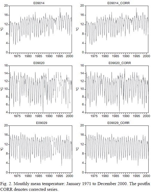
]]> Figure 1 shows the monthly mean temperatures of the 15 stations with more recent data. At least two of them (E09022, E09026) have obvious homogeneity issues, perhaps due to measurement problems, 10 series have large gaps (longer than a year) of missing data and just three have records with an "acceptable" amount of missing data (E09014 lacks seven values, E09020 lacks 26 and E09029 lacks 12). Despite the fact that only three series from ERIC III met our criterion, they are located in three of the four sub-regions defined in Estrada et al. (2009) and represent a considerable portion of MC. That is, series E09029 corresponds to sub-region S1, E09014 to S2 and E09020 to S3. These sub-regions are located in the most urbanized part of the city, where the costs of climatic changes associated to, say, an increase in energy demand, could be higher. The only sub-region not represented in the study (S4) is that with highest elevation and forest areas.3.3 Preliminary data analysis To estimate the missing values and complete the series we used a heuristic procedure based on a linear regression model with deterministic re-gressors such as dummy variables for seasonality and linear trend, when found statistically significant, as it happened with E09014 and E09029. An alternative, formal procedure for estimating missing data is the Time Series Regression with ARIMA Noise, Missing Observations and Outliers (TRAMO) program (Gómez and Maravall, 1996) available at the Bank of Spain website. It is worth noticing that for the time series analyzed here, both procedures lead to similar results. We used CUSUM, CUSUMQ and Quandt-Andrews tests to detect structural changes in the series. Series E09029 required four-step variables to model level changes in: June, 1976 with an increase of 0.96 °C; February, 1980 with a decrease of 1.70 °C; April, 1986 with increase of 1.07 °C; and January, 1996 with a decrease of 0.62 °C. All the dummy variables were significant at the 1% level. Once the series were completed, we improved on the estimation of missing data by applying auto regressive and moving average (ARMA) models, as well as a preliminary VAR model to capture the dynamic relationships among series.
Figure 2 shows the original and completed series E09014, E09020 and E09029 for January 1971 to December 2000 (sample size N = 360). We should notice that the estimated data are considered as known values, so that by taking into account its uncertainty the forecast variance would be larger than that reported here, but the amount of variance attributable to the estimation procedure is unknown.
We started modeling the time series by applying augmented Dickey-Fuller (ADF) unit root tests with centered dummy variables to capture seasonal effects, as in Guerrero (2007). The critical values of the usual ADF test do not change by including this type of dummies. Instead of using data dependent methods as the Akaike or Schwarz criteria (Greene, 2002) we used the Breusch-Godfrey LM and Ljung-Box's Q tests (Enders, 2003) in the auxiliary regressions of the ADF test to select the number of lags required so that the residuals do not show autocorrelation.
To select the deterministic regressors we recall (Enders, 2003) that the unit root tests are conditional on the regressors and the significance of those re-gressors in the model depend on whether or not the series has unit roots. In fact, Campbell and Perron (1991) showed that when the model has more deterministic regressors than the true data generating process, the power of the tests decreases. On the other hand, when the regression model misses a trend component present in the true data generating process, the power of the test goes to zero. Similarly, if the intercept is omitted the power will also decrease. We first decided on the type of deterministic regressors to be included in the ADF tests by looking at the data and followed the procedure suggested by Dolado et al. (1990) when the data generating process is unknown. The general specification of the auxiliary regression was
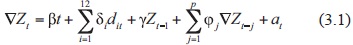
where Zt denotes a monthly mean temperature, t is a linear trend, dit are the centered seasonal dummies and the lags of ∇Zt are used to account for error autocorrelation. The parameters β, δi, φi,- and y are fixed but unknown.
As shown in Table I, the null hypothesis of unit root is strongly rejected for all series, with statistical significance lower than 1% in all cases. The seasonal dummies were also highly significant as well as the linear trend for series E09014 and E09029, with a positive slope in the first case and negative in the second one.1 So, it can be concluded that those series are well represented as trend stationary processes and E09029 as a stationary process with constant mean, therefore there is no need of taking differences to make the series stationary. This is in agreement with previous works (Gay et al., 2007, 2009; Estrada et al. 2010, 2013b; Estrada and Perron, 2014) where the statistical time series analysis lends strong support to the assumption of trend stationary processes to represent monthly or yearly temperature series.
]]>
3.4 VAR model building
Once the order of integration was decided we searched for an appropriate order of the VAR model.2 The estimation results were obtained for January 1971-December 1998, leaving out two whole years of the sample for evaluating the forecasting ability. We decided the order of the VAR(P) model with the criterion of building statistically adequate models as advocated by Spanos (1999). To that end we applied a battery of misspecification tests to validate the assumptions of no error autocorrelation, normality, homoscedasticity and stationarity. This allows being confident that statistical inferences drawn from the model are appropriate (see also Andreou and Spanos, 2003). The resulting order that satisfies the aforementioned assumptions is P = 3, but for comparative purposes we also applied some other criteria to select the value of P, such as likelihood ratio (LR) tests, final prediction error (FPE), Akaike (AIC), Schwarz (SIC) and Hannan-Quinn (HQ). Table II allows us to see that each of these five criteria leads to choosing P < 3, but none of them produces a statistical adequate model. The third lag in the VAR(3) model is not statistically significant in any of the three equations involved, so that the resulting model can be considered slightly over parameterized, but we decided to use P = 3 in order to fulfill the probabilistic model assumptions.
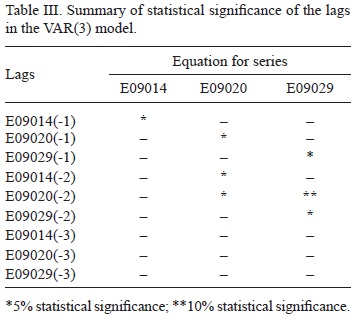
In Table III we can see that the first lag is significant only in the equation for the variable in turn. With regard to second lags: that of E09014 is significant only on E09020; E09020 has a significant effect on itself at the 5% level and on E09029 at the 10% level; E09029 has significant effects on itself only. The third lag is not significant even at the 10% level (the calculated t statistics are between 1.41 and 0.02 in absolute value).
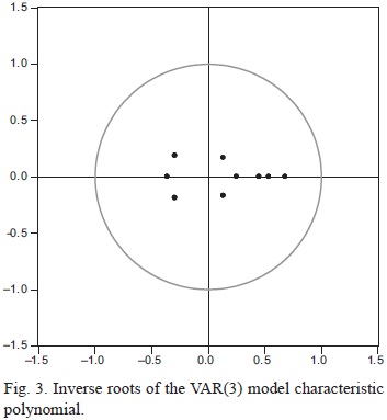
To validate the stationarity assumption of the model we calculated the nine inverse roots of the characteristic polynomial. As shown in Figure 3, all these inverse roots are well inside the unit circle, so that the model can be considered stable.
Avisual inspection ofthe model residuals in Figure 4 is useful to see that there are several possible outlying observations, but the variance does not change systematically. Thus, to validate the homoscedasticity assumption we applied White's test, that is, an omnibus test usually applied to detect heteroscedasticity in general, as proposed in Lutkepohl (2005). The joint test incorporating cross-terms yielded a calculated chi-squared test statistic equal to 458.46 (with p-value 0.000) in such a way that the null hypothesis of error homoscedasticity was rejected. We attribute this result to the possibility of having outlying observations, rather than true heteroscedasticiy.
As previously said, Figure 4 allows to see that several outlying observations are present in the data that can also lead to rejecting the normality assumption. To check the validity of this assumption we applied a multivariate extension of Jarque-Bera's test shown in Lutkepohl (2005), with residuals orthogonalized via Cholesky's decomposition. Table V shows that the null hypothesis of individual normality is rejected by series E09020 and E09029, hence joint normality is rejected too. This fact is basically due to the excess kurtosis in both series and asymmetry in the latter. Since this problem may originate by the presence of outliers, we included some dummy variables to capture the outlying effects.
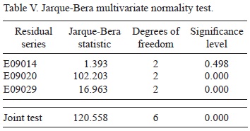
The outliers appear mostly in years where an El Niño/Southern Oscillation (ENSO) occur, be it an El Niño or a La Niña event (Table VI). ENSO is a coupled phenomenon concerning global climatic variability in interannual time scales (Wolter and Timlin, 1998). The literature on this topic has established the existence of some teleconnections of ENSO with weather in several zones of the world (e.g., Glantz, 2001a, b) and its effect on climatic variables in Mexico has also been documented (Magaña, 2004).


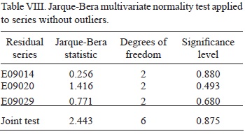
In Table VIII we can observe that once the effects ofthe ENSO events were accounted for the normality assumption is no longer rejected by the Jarque-Bera test. Moreover, the homoscedasticity assumption is also reasonable valid since the joint White test with cross-terms yields a calculated chi-square statistic of 441.56, with p-value of 0.603. Another possibility to correct for excess of kurtosis could have been the use of a heavy tail distribution, such as Student's t, in place of a normal distribution for the errors. That is, by using a t distribution we could have accounted for heavy tails, but that fact does not improve forecasting ability. Thus, that possibility was ruled out because the VAR model will only be used to generate forecasts.
Finally, it is convenient to say that the VAR(3) model provides a better fit for series E09020 (with adjusted R2 = 0.46), than for the other two series, since the corresponding adjusted R2 values are 0.27 for E09014 and 0.29 for E09029.
4. Statistical downscaling for local monthly temperatures in Mexico City
4.1 Evaluating predictive performance and generating scenarios for 2020 and 2100
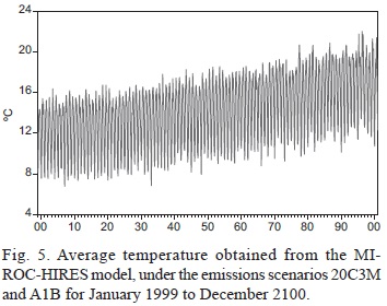
]]> Since the objective of the VAR(3) model in the previous section is to produce climate change scenarios for a much finer spatial scale than climate models can provide, it is important to evaluate its predictive ability in terms of precision and accuracy. In this section, the performance of the out-of-sample one-step ahead forecasts for the period January 1999 to December 2000 is evaluated for both the VAR(3) model without external information (unrestricted forecasts) and the VAR(3) model using information obtained from climate models (restricted forecasts).The external information (Y) used to generate the restricted forecasts is the large-scale (1 x 1° longitude latitude grid point) of the monthly mean temperature from the MIROC-HIRES AOGCM. The selected grid point has its center at -99° E, 18.505° N and covers Mexico City. Two emissions scenarios were used for this purpose: the 20C3M, which aims to reproduce the 20th century climate and the A1B for the 20012100 period (Fig. 5). All climate model simulations were taken from the Climate Explorer of the Royal Netherlands Meteorological Institute (http://climexp.knmi.nl/). The restrictions imposed assume that the average of the three series of observed temperature equals the value of the temperature obtained by the large-scale climate model. Thus, the matrix C is associated with the constraints and defined as a block of diagonal dimension M x kH, where its diagonal contains the vector c = (1/3,1/3,1/3).
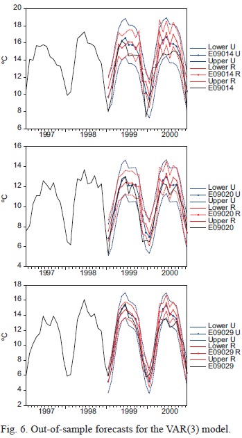
To evaluate the out-of-sample predictive ability of the VAR(3) model the mean error (ME) and the root mean square error (RMSE) were used and the Diebold-Mariano (DM) test was applied to determine whether there is a significant difference between restricted and unrestricted forecasts. The ME is a measure of forecast accuracy: positive values indicate that on average the forecast values are higher than the observed ones, while negative values indicate that on average forecasts are below the observed values. The RMSE is a measure of precision for which values closer to zero indicate a better forecast. The DM test compares the prediction precision of two sets of forecasts. Some of the advantages of this test are that it allows the forecast errors to be non-normal, to have a non-zero mean, to be serially and contemporaneously correlated (Diebold and Mariano, 1995). As shown in Table IX, the unrestricted forecasts are more accurate and precise than restricted for all series.
For the E09014 forecast, the magnitude of the ME is larger than those of other series, and thus a greater overestimation can be expected for this series. The E09014 forecasts (restricted and unrestricted) have lower precision than those of E09020 and E09029 (Fig. 6). The differences in the values of ME and RMSE between both types of forecasts are small, in the sense that they are lower than one degree Celsius. Moreover, the DM test (Table IX) provides formal evidence suggesting that the restricted and unrestricted forecasts are not statistically different.
While it could be argued that the external information obtained from the MIROC-HIRES model does not improve the VAR(3) model forecasts in the short term, it is essential for the medium and long term projections since it allows indirectly to incorporate the effect of external forcings which would be omitted in the unrestricted forecasts. Additionally, the compatibility of the forecasts generated by the VAR(3) and the external information used to restrict forecasts was evaluated. The total compatibility test proposed in Guerrero et al. (2008) yields a value Kcalc= 0.872 (probability of 0.640), which suggests that the two sources of information are compatible. Similarly, a partial compatibility test shows that the information from both sources is compatible with all the imposed constraints.
4.2 Local climate change scenarios for 2020 and 2100 based on restricted forecasts
]]> In this subsection the restricted forecasts —which include the additional information from the climate model-HIRES MIROC— are compared to those from the unrestricted VAR(3) model. Figures 7 and 8 show the unrestricted (left) and restricted (right) forecasts for 2020 and 2100, respectively. The prediction intervals do not grow over time because the processes are trend-stationary (E09014 and E09029) and stationary around a constant (E09020). However, in practice for long forecast horizons a larger uncertainty could be expected as the forecast horizon grows because of, for example, potential parameter instability (i.e., these forecasts do not consider epistemic uncertainty; see Gay and Estrada, 2010).For the period comprising January 2001 to December 2020, the restricted (unrestricted) forecasts show an increase of 2.64 °C (2.51 °C) for E09014, a cooling of 0.27 °C (0.36 °C) for E09029 and a no significant trend for E09020. For this forecast horizon and in the case of E09014 and E09029, the restricted forecasts imply higher temperatures than the unrestricted ones. For this forecast horizon, the total compatibility test statistic yields a value of 0.815 for which, using the normal approximation, it can be concluded that the sources of information used for forecasting are compatible.3 The partial compatibility tests show that the sources are compatible at the 5% level, except for restrictions 16 and 115.
While the large-scale temperature produced by the MIROC-HIRES shows an increase of 5.37 °C from January 2001 to December 2100, the restricted forecasts from the VAR(3) model indicate that for the same period E09029 would experience a cooling of 0.38 °C, E09014 an increase of14.80 °C and E09020 a rise of 1.70 °C. In the case of the unrestricted forecasts, E09014 would experience a warming of 12.29 °C, E09020 would remain unchanged and E09029 would decrease 2.16 °C. The effects of the restriction imposed by the MIROC-HIRES model are particularly noticeable for E09029, in which the cooling is about 82% smaller than that obtained by the unconstrained forecast. That is, when the external forcings are taken into account (i.e., the A1B emissions scenario used for running the climate model) and not just the extrapolation of the trend included in the VAR(3) model, the effects of the local factors responsible for cooling are partially offset by the larger-scale warming caused by climate change. This can be observed in Figure 8c, in which the negative trend becomes less pronounced after midcentury.
When the forecasts are restricted using the climate model output, the mean of E09020 is no longer a constant mean, as it shows a moderate warming trend towards the end of the century. In the case of E09014, the restricted forecasts have a mean value in 2100 more than two degrees Celsius higher in comparison with the unrestricted forecasts. Figures 7 and 8 show another important effect of restricting the forecasts to the climate output: the variability shown by the forecasted series is similar to that ofthe observations. The total compatibility test for the restricted forecasts for the period January 2001 to December 2100 has a value of 2.99, which indicates that the sources of information used for forecasting are compatible. The partial compatibility tests show less compatibility between the two sources of information: in 272 cases the null hypothesis of compatibility is rejected at the 5% significance level.
The results are consistent with the sub-regions where the stations are located as the differences in warming between them reflect local anthropogenic and natural factors that affect the climate of the city: the strongest warming occurs in E09014, which represents the most urbanized sub-region and the warming can be explained as a joint product of the increase in regional temperature due to climate change and to the heat island phenomenon caused by urbanization; the E09020 station shows a lower increase in temperature than E09014 due to a smaller contribution of local factors; a possible explanation for the decrease in the observed and forecasted temperatures in the E09029 sub-region could be that it is located in the industrial area of the city. Industrial activity produces large amounts of atmospheric aerosols that have a negative effect on radiative forcing, causing a decrease in local and even regional temperatures (e.g., Jin et al., 2010). However, it should be noted that the results indicate thermal contrasts that can hardly be observed among neighbor sub-regions located within such a small area. Therefore, in the next sections we propose a new approach that can lead to results that are more consistent with the physics of climate and with the observed differences in local microclimates.
For the purposes of what is discussed below, it is important to underline the differences between climate forecast and climate scenario. Climate forecasts aim to estimate the true evolution of future climate, and the dominant uncertainty in this case is randomness. By contrast, a climate scenario is a possible, self-consistent and simplified representation of the potential evolution of future climate dependent on (or conditioned by) a set of key variables that are inherently uncertain. In this case, the type of uncertainty is primarily epistemic (IPCC, 2007; Gay and Estrada, 2010). As such, it is appropriate to interpret the results of any downscaling of climate change as conditional on a number of assumptions that are made about both the local (e.g., land use and deforestation, among others), regional (e.g., regional climate patterns) and global determinants (e.g., global climate, concentrations of greenhouse gases). The future evolution of all these conditioning factors is subject to epistemic uncertainty.
4.3 Local climate change scenarios for 2020 and 2100 corrected by changes in local factors
The results shown in the previous subsection portrait one of the main limitations of most downscaling applications, irrespective of whether a dynamic or statistical approach is used. The general framework for downscaling methods described by y = f (X, l, G) —for which the local climate is a function of the local physiographic effects, large-scale factors and global characteristics— is replaced in practice by y =f'(X) that assumes the effects of all local factors (as well as of the changes in the global climate) to be constant, limiting the local climate to be a function ofy and X exclusively. As argued below, local climate change scenarios can hardly be considered realistic or useful if the effects of local factors are simply extrapolated (as is currently done in most downscaling exercises) into the future without stating the underlying assumptions that are being made. The assumed evolution of local factors should be clear to the potential users as is required with other forcings. If this condition is not met, the local climate change scenario would be essentially meaningless, as would be a global climate change scenario for which no information is given regarding its radiative forcing drivers.
The effects of urbanization on the climate of cities have been discussed in the literature and it has been shown that these effects can generate both large warming and cooling trends. However, the urbanization processes can be limited by different factors such as physical constraints and urban planning and policy (i.e., when a city is completely urbanized, or an urbanization goal is reached). Consequently, the warming/cooling caused by these factors would tend to stabilize at some level instead of showing a constant growth. Clearly, extrapolating their effects by means of trends with constant slope parameters would be unrealistic and in many cases physically impossible when long horizons are considered (as is the case of climate change projections). Thus, the cooling shown by E09029 or the large warming shown by E09014 could be overestimated as they assume constant rates of urbanization and air pollution, which are probably impossible in reality. Likewise, it could be argued that the warming in E09020 may be underestimated given that the areas at piedmont may show in the future higher rates of urbanization than what has been previously observed. However, how to integrate these changes for producing local climate change scenarios is currently a subject of discussion in the downscaling literature and most of the current downscaling applications simply ignore this problem (IPCC, 2007).
To address this issue, we propose a simple approach for distinguishing the contributions of large-scale and local factors to the observed trends in local temperatures. This decomposition allows creating more credible and physically consistent projections. Assume that the slope of the trend of a temperature series can be expressed as follows
]]>
where βLSF is the slope that can be attributed to large scale factors and βLF represents the effects of the local scale factors. Furthermore, if βLSF can be approximated by the large-scale (X) temperature (i.e., a grid point or points encompassing the area to be downscaled) the effects of local and large-scale factors can be separated. The large-scale data can be obtained either from (1) a gridded dataset of observed variables or (2) the output of a climate model.4 By means of this decomposition, instead of extrapolating the part of the trend that can be attributed to local factors, a scenario representing the possible evolution of local factors can be introduced. As before, the large-scale factors are represented by the output of a climate model, and both sources of information are integrated using restricted forecast techniques to create a local climate change scenario.
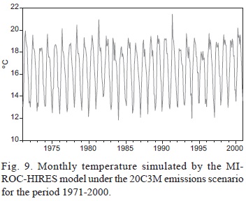
Figure 9 shows the monthly temperature simulation corresponding to the MIROC-HIRES for the 20C3M emissions scenario covering the period 1971-2000. As can be seen from this figure, the large-scale temperature series (1 x 1°) for the grid point encompassing the area of study does not show a trend; instead it oscillates around a constant mean value. Using a linear regression with a time trend as explanatory variable it is confirmed that the slope coefficient is not statistically different from zero (p-value 0.211).5 However, this p-value should be seen cautiously because the autocorrelation structure in the series was not accounted for by the trend model. Taking the MIROC-HIRES simulation as the representation of the contribution of the large-scale factors to the observed local warming it can be argued that pLS1F = 0 during the period of study. Consequently, the observed trends in E09014 y E09029 could be attributed solely to the effects of local factors and not to global climate change or to any other large-scale phenomenon. Clearly these conclusions could vary if a different database (observed or simulated) is used to represent the behavior of the large-scale temperature over this period.
The local factors with largest influence over the local climate of Mexico City are the urban heat island generated by the urbanization processes in the sub-region represented by E09014 and the effect of atmospheric aerosols produced by the industrial area located in the sub-region represented by E09029. In the case of E09020, the local factors did not generate significant trends during the period of study. Given the current level of urbanization shown in the E09014 sub-region it is reasonable to assume that at the latest in the medium term, the levels of urbanization and warming caused by this phenomenon will approach zero and the temperature will tend to stabilize at some level (higher than its present value). Similarly, the cooling trend, possibly caused by the increase in atmospheric aerosols, will also tend to zero (or might even reverse) in a not too distant future, due to regulations that will probably be adopted to control them due to the effect that these particles have on human health.
To illustrate this method we present an example of local climate change scenarios generated using restricted forecasts in which a structural change in the slope of the trend is induced to represent a scenario of changes in the local policies to control air pollution and to limit further urbanization in the sub-regions E09029 and E09014, respectively. The break date of the structural change is set to January of 2020. Therefore, local factors will continue to increase/ decrease local temperatures at the same rate of the observed period until that date. For the sub-region E09020 it is assumed that local factors will continue to have no effect over the local temperatures (e.g., the levels of atmospheric pollution and urbanization do not change). However, the mid- and long-term temperature changes in the different sub-regions will be driven by the large-scale warming scenario produced by the MIROC-HIRES. These projections can be interpreted as intervention scenarios, in which public policies regarding land cover and land use change, as well as atmospheric pollution control, are used to modify the microclimates of the city, intensifying or reducing some of the impacts of global climate change compared to a non-intervention scenario.
The corrected unrestricted forecasts in Figure 10 (left panel) show the changes in temperatures produced by the evolution of local factors prescribed using dummy variables. Comparing with the unrestricted forecasts in Figure 8, in this case the sub-region E09014 shows a warming of 2.62 °C instead of 12.29 °C for 2100. Note that the difference of about 10 °C in warming is produced only by the assumed evolution of local factors: the first determined by an intervention scenario and the second on an extrapolation of the current trends. As has been discussed in the literature on scenarios generation, the extrapolation of current trends usually leads to physical and socioeconomic inconsistencies (Nakicenovic and Swart, 2000). In the case of the sub-region E09029, the cooling obtained by using the corrected unrestricted forecasts is 0.45 °C instead of the 2.16 °C cooling obtained by means of the uncorrected unrestricted forecasts.
The corrected restricted forecasts (Fig. 10, right panel) show the evolution of temperatures in the three sub-regions represented by E09014, E09020 and E09029. These projections combine the large-scale temperature change obtained by the MIROC-HIRES model under the A1B scenario and the scenario of local factors described above. By 2100 the temperature in the sub-region E09014 shows an increase of 7.46 °C - about half of the warming projected with the uncor-rected restricted forecasts. The increase in temperature in the sub-region E09020 is 4.34 °C and 4.32 °C in the sub-region E09029 (2.64 °C and 4.70 °C higher than those obtained by means of the uncorrected restricted forecasts, respectively). The temperature contrast in the uncorrected forecasts is so large (more than 13 °C) that could be hardly maintained in such a small geographical area such as Mexico City. On the contrary, the corrected restricted forecasts provide a more credible representation of the future climate since the differences in temperatures between regions are much smaller (about 3 °C) in the corrected scenarios and are comparable to the temperature differences that have been observed in the past. Furthermore, it is important to notice that the scenarios based on corrected restricted forecasts are not based on the extrapolation of current trends of local factors (such as high urbanization rates in an already highly urbanized area) that would be impossible to maintain for the long-term horizons used for climate change projections. The extrapolation of local trends is implied by the available statistical downscal-ing methods that have been proposed for producing climate change scenarios (Benestad et al., 2008).
]]> 5. Conclusions
This work considers the generation of scenarios of climatic change for spatial scales much smaller than the current general circulation models can handle and discusses that usually the corresponding statistical methods underlying those techniques are commonly in fault. The approach based on VAR models and restricted forecasting is more appropriate in that: (1) a multivariate model is preferable to capture the relationships among the series involved and offers a better representation at the local level; (2) there is no need of specifying a long-term relationship between large-scale and local-level variables, which could be complicate and generate spurious results; (3) restricted forecasting can produce scenarios with variability similar to that in the observed series (this is something that cannot be obtained with the methods in current use); (4) we can test for compatibility between information coming from historical records and that produced by general circulation models.
The scenarios generated in this work are based on statistically adequate models, so that inferences can be drawn on solid grounds, in contrast with usual inferences derived from techniques based on numerical optimization criteria. It is also important to distinguish between local factor contributions and those of large-scale when considering trends in climatic time series. This point is relevant since current downscaling methods incorporate the evolution of global or regional factors, but assume that the local warming/cooling observed rates stay constant for all time horizons. Such an assumption implies that the rate of change of local factors (e.g. urbanization) remains constant, which is untenable in most cases.
As it happens with global and regional projections of climatic change derived from general circulation models and large scale-forcing, it is required to propose a possible evolution for the effect of local forcing, particularly when long horizons are considered. This should be done on the basis of a scenario of evolution of local factors supported by an estimation of their effects on local climate. In order to do that, we proposed a simple method to separate local from large-scale effects, by means of dummy variables that affect the part of the slope attributable to local forcing. If such a correction is not applied, the resulting local scenarios show temperature contrasts very far to what is expected in neighbor sub-regions within such a reduced area. In addition, by selecting different evolution patterns that represent, for instance, different public policies about land use or pollution control, the suggested methodology offers the possibility of evaluating the convenience of such policies, with regard to their effects for amplifying or attenuating the impact of climatic changes.
Acknowledgements
Víctor M. Guerrero gratefully acknowledges the financial support provided by Asociación Mexicana de Cultura, A. C. to carry out this research. Francisco Estrada acknowledges financial support for this work from the Consejo Nacional de Ciencia y Tecnología (http://www.conacyt.gob.mx) under grant CONACYT-310026, as well as from PASPA-DGAPA of the Universidad Nacional Autónoma de México.
References
Andreou A. and A. Spanos, 2003. Statistical adequacy and the testing of trend versus difference stationarity. Economet. Rev. 22, 217-237. [ Links ]
Benestad R. E., I. Hanssen-Bauer and D. Chen, 2008. Empirical-statistical downscaling. World Scientific Publishing Company, 228 pp. [ Links ]
Bravo J. L., C. Gay, C. Conde and F. Estrada, 2006. Probabilistic description of rains and ENSO phenomenon in a coffee farm area in Veracruz, Mexico. Atmósfera 19, 49-74. [ Links ]
Campbell J. Y. and P. Perron, 1991. Pitfalls and opportunities: What macroeconomists should know about unit roots. In: NBERMacroeconomics Annual 1991, vol. 6 (O. J. Blanchard and S. Fischer, Eds.). MIT Press, Cambridge, pp. 141-220. [ Links ]
CONAPO, 2002. Implicaciones demográficas y territoriales de la construcción de un nuevo aeropuerto en la ZMVM. Serie Documentos Técnicos. Consejo Nacional de Población, Mexico. [ Links ]
Conde C., F. Estrada, B. Martínez, O. Sánchez and C. Gay, 2011. Regional climate change scenarios for Mexico. Atmósfera 24, 125-140. [ Links ]
Diebold F. X. and R. Mariano, 1995. Comparing predictive accuracy. J. Bus. Econ. Stat. 13, 253-265. [ Links ]
Dolado J. J, T. Jenkinson and S. Sosvilla-Rivero, 1990. Cointegration and unit roots. J. Econ. Surv. 4, 249-273. [ Links ]
Enders W., 2003. Applied econometric time series. 2nd ed. Wiley, New York, 480 pp. [ Links ]
Estrada F., A. Martínez-Arroyo, A. Fernández-Eguiarte, E. Luyando and C. Gay, 2009. Defining climate zones in Mexico City using multivariate analysis. Atmósfera 22, 175-193. [ Links ]
Estrada F., C. Gay and A. Sánchez, 2010. Reply to "Does temperature contain a stochastic trend? Evaluating conflicting statistical results", by Kaufmann et al. Climatic Change 101, 407-414, doi:10.1007/s10584-010-9928-0. [ Links ]
Estrada F., V. M. Guerrero, C. Gay and B. Martínez, 2013a. A cautionary note on automated downscaling methods for climate change. Climatic Change 120I, 263-276, doi:10.1007/s10584-013-0791-7. [ Links ]
Estrada F., P. Perron and B. Martinez, 2013. Statistically derived contributions of diverse human influences to twentieth-century temperature changes. Nat. Geosci. 6, 1050-1055, doi:10.1038/ngeo1999. [ Links ]
Estrada F. and P. Perron, 2014. Detection and attribution of climate change through econometric methods. Bol. Soc. Mat. Mex. 20, 107-136. [ Links ]
Gay C., F. Estrada and C. Conde, 2007. Some implications of time series analysis for describing climatologic conditions and for forecasting. An illustrative case: Veracruz, Mexico. Atmósfera 20, 147-170. [ Links ]
Gay C., F. Estrada and A. Sánchez, 2009. Global and hemispheric temperatures revisited. Climatic Change 94, 333-349. [ Links ]
Gay C. and F. Estrada, 2010. Objective probabilities about future climate are a matter of opinion. Climatic Change 99, 27-46, doi: 10.1007/s10584-009-9681-4. [ Links ]
Giorgi F., B. Hewitson, J. Christensen, M. Hulme, H. von Storch, P. Whetton, R. Jones, L. Mearns and C. Fu, 2001. Regional climate information - evaluation and projections. In: Climate change 2001: The scientific basis. Contribution of Working Group I to the Third Assessment Report of the Intergovernmental Panel on Climate Change (J. T. Houghton, Y. Ding, D. J. Griggs, M. Noguer, P. J. van der Linden, X. Dai, K. Maskell and C. A. Johnson, Eds.). Cambridge University Press, Cambridge, United Kingdom and New York, pp. 585-638. [ Links ]
Glantz M., 2001a. Once burned, twice shy? Lessons learned from the 1997-98 El Niño. United Nations University Press, New York, 28 pp. [ Links ]
Glantz M., 2001b. Currents of change. Impacts of El Niño and La Niña on climate and society. Cambridge University Press, 268 pp. [ Links ]
Gómez V. and A. Maravall, 1996. Programs TRAMO and SEATS. Instructions for the user (with some updates). Working Paper 9628, Research Department, Banco de España, 122 pp. [ Links ]
Greene W. H., 2002. Econometric analysis, 5th ed. Prentice Hall, 1026 pp. [ Links ]
Guerrero V. M., 2007. Pronósticos restringidos con modelos de series de tiempo múltiples y su aplicación para evaluar metas de política macroeconómica en México. Estudios Económicos 22, 241-311. [ Links ]
Guerrero V. M., B. Pena, E. Senra and A. Alegría, 2008. Restricted forecasting with a VEC model: Validating the feasibility of economic targets. Estadística 60, 83-101. [ Links ]
Guerrero V. M., E. Silva and N. Gómez, 2013. Building scenarios of multiple time series that take into account the effects of an expected intervention. J. Forecast. 33, 32-46, doi:10.1002/for.2271. [ Links ]
IPCC, 2007: Climate change 2007: The physical science basis. Contribution of Working Group I to the Fourth Assessment Report of the Intergovernmental Panel on Climate Change (S. Solomon, D. Qin, M. Manning, Z. Chen, M. Marquis, K. B. Averyt, M. Tignor and H. L. Miller, Eds.). Cambridge University Press, Cambridge, United Kingdom and New York, 996 pp. [ Links ]
Ishi A., S. Iwamoto, T. Katayama, T. Hayashi, Y. Shiotzuki, H. Kitayama, J. Tsutsumi and M. Nishida, 1991. A comparison of field surveys on the thermal environment in areas surrounding a large pond: When filled and when drained. Energ. Buildings 15-16, 965-971. [ Links ]
Jáuregui E., 1991. Effects of revegetation and new artificial water body on the climate of northeast Mexico City. Energ. Buildings 15-16, 447-455. [ Links ]
Jáuregui E., 2000. El clima de la ciudad de México. Instituto de Geografía, UNAM/Plaza y Valdés, Mexico, 131 pp. [ Links ]
Jin M., J. M. Shepherd and W. Zheng, 2010. Urban surface temperature reduction via the urban aerosol direct effect: A remote sensing and WRF model sensitivity study. Advances in Meteorology, doi:10.1155/2010/681587 [ Links ]
Jones P. D., P. Y. Groisman, M. Coughlan, N. Plummer, W. C. Wang and T. R. Karl, 1990. Assessment of urbanization effects in time series of surface air temperature over land. Nature 347, 169-172. [ Links ]
]]>Lütkepohl H., 2005. New introduction to multiple time series analysis. Springer-Verlag, 764 pp. [ Links ]
Magaña R. V. (Ed.), 2004. Los impactos del niño en México. Centro de Ciencias de la Atmósfera, UNAM/ Secretaría de Gobernación, Mexico, 229 pp. [ Links ]
Nakicenovic N. and R. Swart (Eds.), 2000. Special report on emissions scenarios. Cambridge University Press, 570 pp. [ Links ]
Peña D., G. C. Tiao and R. S. Tsay, 2001. A course in time series analysis. John Wiley, New York, 460 pp. [ Links ]
Sims C. A., 1980. Macroeconomics and reality. Econometrica 48, 1-48. [ Links ]
]]>Spanos A., 1999. Probability theory and statistical inference: Econometric modeling with observational data. Cambridge University Press, 815 pp. [ Links ]
Von Storch H., E. Zorita and U. Cubasch, 1993. Down-scaling of global climate change estimates to regional scales: An application to Iberian rainfall in wintertime. J. Climate 6, 1161-1171 [ Links ]
Von Storch H., B. Hewitson and L. Mearns, 2000. Review of empirical downscaling techniques. In: Regional climate development under global warming (T. Iversen and B. A. K. Hoiskar, Eds.). General Technical Report 4. Available at: http://regclim.met.no/rapport_4/presentation02/presentation02.htm. [ Links ]
Wei W. W. S., 1990. Time series analysis: Univariate and multivariate methods. Addison-Wesley, Redwood City, CA, 478 pp. [ Links ]
Wilby R. L. and T. M. L. Wigley, 1997. Downscaling general circulation model output: A review of methods and limitations. Prog. Phys. Geog. 21, 530-548. [ Links ]
Wilby R. L. and T. M. L. Wigley, 2000. Downscaling general circulation model output: A reappraisal of methods and limitations. In: Climate prediction and agriculture (M. V K. Sivakumar, Ed.). Proceedings of the START/ WMO International Workshop, Geneva. International START Secretariat, Washington, pp. 39-68. [ Links ]
Wilby R. L., S. P. Charles, E. Zorita, B. Timbal, P. Whetton and L. O. Mearns, 2004. Guidelines for use of climate scenarios development from statistical downscaling methods. Supporting material of the Intergovernmental Panel on Climate Change. Available from the IPCC Data Distribution Center of the Task Group on Climate Change Impacts Assessment, 27 pp. [ Links ]
Wolter K. and M. S. Timlin, 1998. Measuring the strength of ENSO events - how does 1997/98 rank? Weather 53, 315-324. [ Links ]
Zivot E. and J. Wang, 2005. Modeling financial time series with S-PLUS, 2nd ed. Springer, 998 pp. [ Links ]
1 Afterwards, the trends were estimated correcting for autocorrelation and verifying parameter stability by means of CUSUM, CUSUMQ and Quandt-Andrews tests. Series E09014 has a positive trend of 1.12 °C/decade, whereas E09029 has a negative trend of 0.21 °C/decade.
2 The effects of the deterministic trend and seasonal dummies were removed from the series in order to produce forecasts with a VAR model as indicated by Lutkepohl (2005).
]]> 3 Given the large number of degrees of freedom due by the length of the forecast horizon, the x2 probability cannot be computed and therefore a normal approximation has to be used instead.4 Note that local temperature forms part of the grid point representing the large-scale temperature average. However, the influence of a single point over hundreds of squared kilometers that usually make up a grid point is practically zero.
5 CUSUM, CUSUMQ and Quandt-Andrews tests for structural change were applied to evaluate the presence of a potential structural change in the slope of the trend. None of the tests provided significant evidence in favor of a structural break.
]]>