J. D. GÓMEZ DÍAZ, A. I. MONTERROSO RIVAS, J. A. TINOCO RUEDA, M. L. TOLEDO MEDRANO
Departamento de Suelos, Universidad Autónoma Chapingo,
km 38.5 Carretera México–Texcoco, Chapingo, 56230, Estado de México.
Corresponding author: J. D. Gómez Díaz; e–mail: dgomez@correo.chapingo.mx

C. CONDE ÁLVAREZ and C. GAY GARCÍA
Centro de Ciencias de la Atmósfera, Universidad Nacional Autónoma de México,
Circuito Exterior, Ciudad Universitaria, México, D. F., 04510, México

RESUMEN

Se analizaron los impactos del cambio climático en el sector forestal mediante simulaciones en la distribución potencial de 16 especies forestales en la República Mexicana, para zonas templadas, tropicales y semiáridas. Se estudiaron para el escenario base así como para tres modelos de cambio climático (GFDL–CM–2.0, MPI–ECHAM–5, HADGEM–1) bajo los escenarios de emisiones socioeconómicos A2 y B2 al horizonte de tiempo 2050. La metodología consistió en: 1) modelación de la climatología en el periodo 1950–2000 (escenario base), 2) aplicación de razones de cambio de los tres modelos de cambio climático, 3) cálculo del balance de humedad en el suelo, 4) creación de matrices de requerimientos ambientales de las especies forestales y 5) simulación de la distribución potencial espacial de las especies. Los resultados obtenidos muestran que todas las especies forestales de las zonas templadas se verán afectadas para el horizonte de tiempo considerado, como consecuencia del incremento en la temperatura en todo el territorio nacional y la disminución de la precipitación en casi todos los meses del año. En las especies de zona tropical, con excepción de Cedrela odorata, se presenta una disminución considerable en los niveles de mayor aptitud, lo que se asocia a restricciones para su desarrollo al incrementarse el periodo seco, asimismo, las áreas templadas, que tendrán un aumento en la temperatura, serán de aptitud limitada para estas especies. Para las especies de la región semiárida y árida, los modelos reportan que se espera un incremento de la superficie sin aptitud, lo que se asocia al incremento del déficit hídrico y en las zonas que actualmente se consideran marginales las restricciones serán más severas. De los modelos de cambio climático considerados, el HADGEM–1 establece las condiciones más restrictivas, el MPI–ECHAM–5 establece una situación intermedia de afectación negativa y el modelo GFDL–CM–2.0 establece incrementos de la superficie con cierto grado de aptitud. Geográficamente, el país no presenta cambios constantes en la distribución potencial de las especies, estas varían de acuerdo al modelo de cambio climático utilizado, la especie analizada y la zona ecológica delimitada.

ABSTRACT

In order to analyze the impacts of climate change on species endowed with forestry relevance, the present study practiced simulations in the potential distribution of 16 forest species inside the Mexican Republic's temperate, tropical, and semiarid zones. For the examination of this effect we pictured the base scenario, as well as three models of climate change (GFDL–CM–2.0, MPI–ECHAM–5, HADGEM–1) that would take place under the socio–economic scenarios A2 and B2 by 2050. The methodology consists in: 1) a modeling of climatology corresponding to the period 1950–2000 (base scenario); 2) a consideration of the reasons for the change in precipitation and temperature within each one of the three climate change models; 3) a calculation of the soil humidity balance; 4) the creation of matrices of the forest species' environmental requirements, and 5) a proposal for a potential spatial distribution of the species. The results show that, because of a rise in temperature and a decrease in precipitation along the entire national territory almost every month, each one of the forest species living in the temperate zones will be affected within the span of time considered. Among the species of the tropical zones, there appears a substantial decrease in the levels of those with the highest suitability, which is linked to the restrictions that are set on their development as the dry period is heightened. As for the species of the arid and semi–arid regions, the models indicate that an increase will be marked on the area of those with no suitability, which is associated with the enhancement of hydric deficit. Of the climate change models here considered, the HADGEM–1 establishes the most restrictive conditions, the MPI–ECHAM–5 establishes an intermediate situation of affectation, and the model GFDL–CM–2.0 establishes the least affectation. Geographically, the country does not present constant changes in the potential distribution of the species; these latter vary according to the climate change model that has been used, the species that has been analyzed, and the ecological zone that has been delimited.

Keywords: forestry sector, general circulation models, climate change scenarios, forest land suitability, México.

1. Introduction

There are different methodologies to simulate the potential distribution of species or of flora and fauna communities (Naoki et al., 2006). Currently, by means of the techniques of remote perception and geographic information systems, more detailed results within a shorter term can be obtained. Some of the best–known models of simulation are: GARP (Genetic Algorithm for Rule–set Prediction), a heuristic system based on artificial intelligence that is in pursuit of non–random correlations between the organism's points of presence and the environmental variables (Stockwell and Peterson, 2002); and BIOCLIM (Busby, 1991), a model that grants the species the ecological range of n predictive variables it has generated, through an analysis of the distribution of the registers of presence fixed upon each environmental variable (Benito and Peñas, 2007). Now, even though these models have been applied on a regional and national scale in some countries, it is undeniable that, if the simulations are to be triggered, a set of reliable field data is still needed (Manel et al., 2001; Anderson et al., 2003; Téllez et al., 2004; Segurado and Araújo, 2004). There is, however, another cluster of methods based on the principle of the limiting factor and whereby the biggest number of possible ecological variables is characterized, while a certain species' development requirements are met (FAO, 1981; Sys et al., 1993). These two factors are then contrasted and, consequently, it is possible to determine the potential distribution zones for the plant species, which have been categorized by suitability levels. The method submitted by Gómez et al. (2007), which is included in this group, was the one we chose to apply for the zonification of 16 forest species, on the grounds that it fittingly goes along the lines of the general objectives held by the Fourth National Communication submitted by México to the United Nations Framework Convention on Climate Change.

2. Methodology

The methodology that was used, which corresponds to the one proposed by FAO (1981) and Sys et al. (1993) and, simultaneously, takes into account the ameliorations suggested by Gómez et al. (2007), is divided into six phases, namely:

a) Base scenario of climatic variables

The geographical distribution of the temperature and precipitation variables for the base scenario was elaborated by the Centro de Ciencias de la Atmósfera of the Universidad Nacional Autónoma de México. The values of both variables resulted from the average of the data relative to the period 1950–2000. Running parallel to this calculation, and with the aim in mind of being able to use the chosen method, we selected 3770 meteorological stations on a national scale which had been reported by the CLICOM system (WMO, 2007), based on the number of years and the percentage of the reported data.

b) Areas of climatic influence

The areas of climatic influence (ACI) are defined as geographical units that represent the conditions of the annual and monthly temperature and precipitation in a certain region of the earth surface (Gómez et al., 2008), which are obtained from the superposition of the annual mean isotherms and isohyets through the ArcView Geographical Information System (ESRI, 2006).

To draw the isotherms, it was applied a simple method (Ortiz, 1987), which entails creating models of simple linear regression whereby the behavior of temperature vis–à–vis the height of the ground is analyzed. Once the country had been segmented into 25 thermic zones, we proceeded to estimate their models of regression for each month and on a yearly basis; the latter model was applied to the digital elevation model (INEGI, 2008), thereby obtaining the map of annual mean temperature.

After the values of temperature and the annual media precipitation were geographically delimited, the maps of the annual isohyets and isotherms were superimposed. The upshot of this was the formation of 2530 polygons throughout México, which correspond to the ACI.

c) Climate change models

The general circulation models (GCM) we used were the HADGEM–1, the GFDL–CM–2.0, and the ECHAM5–MPI; the socio–economic scenarios that we evaluated were scenarios A2 and B2, which are presumed to be looming by 2050. The GCM have a spatial resolution of 2.5° × 2.5°, and their outlets were obtained by the Centro de Ciencias de la Atmósfera of the Universidad Nacional Autónoma de México (UNAM) (Conde et al., 2008). The change rates in each model were applied to the data of the ACI belonging to the base scenario, wherewith we attained the scenarios for each GCM by 2050.

d) The balance of soil moisture

The balance of soil moisture was made using the Thornthwaite and Matter's (1957) methodology modified version III (Estrada–Berg et al., 2008). While pursuing this balance, the study was based on the monthly mean temperature and the monthly mean precipitation, as well as the soil properties and the kind of vegetation that is developed; thus, it was possible to calculate the soil's moisture storage capacity (MSC). To define whether a month is dry, we created a humidity index (HI) by dividing the precipitation of that month plus the humidity in storage that is used when this happens by the potential evapotranspiration (ET) of the same month. If the HI is >1, the month is considered humid; if it is between 0.5 and 1, the month is intermediate, and if it is < 0.5, it is dry. To determine the humidity balance for the base scenario, we considered the values of monthly mean temperature and precipitation in each one of the ACI, together with the values of PSC for the types of vegetation found in the National Forest Inventory (Inventario Nacional Forestal) which was prepared by UNAM and the Environment and Natural Resources Ministry (Secretaría de Medio Ambiente y Recursos Naturales, SEMARNAT–UNAM, 2001), as well as the soil properties reported by INEGI (2006). In the case of the scenarios of climate change, the humidity balance was carried out applying the ratios of change in temperature and precipitation which were achieved by the models used for each one of the ACI, while considering the same MSC of the base scenario.

e) The potential distribution of forest species

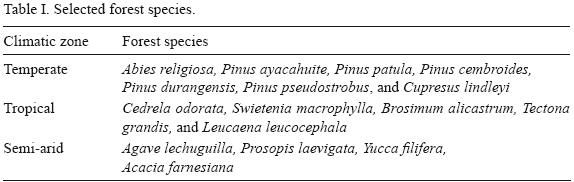
In proportion to their forestry importance, 16 forest species were selected in order to effect the simulation of their potential distribution and the possible transformation of the base scenario into the climate change scenarios. The selected species were grouped in three climatic zones (Table I) which, generally speaking, cover most of the eco–climatic conditions in México. To simulate the potential spatial distribution of the forest species in the scenarios that have been mentioned, we designed matrices of environmental requirements for each species, considering as the principal element the research cards about the conditions of the different species and the environmental components in the sampling point net of the forest species which was distributed by the National Forest Commission (Comisión Nacional Forestal, CONAFOR, 2007). Additionally, documentary and cartographic information was gathered from the following materials: the technical cards relative to the Reforestation Information System (Sistema de Información para la Reforestación, SIRE) which were elaborated by CONAFOR and the National Commission for the Knowledge and Use of Biodiversity (Comisión Nacional para el Conocimiento y Uso de la Biodiversidad, CONABIO, 2006); and the monographies of Mexican pines prepared by the National Institute of Forest, Agricultural, and Livestock Research (Instituto Nacional de Investigaciones Forestales, Agrícolas y Pecuarias, INIFAP) and CONABIO (INIFAP–CONABIO, 2003).

Each one of the matrices was applied to the cartography of the climatic variables in the base scenario and the climate change scenarios, making use of software ArcGIS 9.2. The end–result matrices contain information about ecological variables under which each species is being developed; the values, which are expressed in terms of ranges, were grouped in four categories referring to suitability levels: suitable, moderately suitable, marginally suitable, and not suitable.

In México the temperate zones occupy an area of approximately 46 million hectares, which amounts to 23.4% of the national territory. As far as this ecological zone is concerned, the species that the present study put under scrutiny were: Abies religiosa (Kunth) Schldl. et Cham., or oyamel fir, which is a demanding species in terms of humidity and temperature requirements, and which grows to an altitude of between 2500 and 4000 m above sea level (Madrigal, 1967); Pinus ayacahuite Ehren., or table pine, which is distributed along the pine forests and the pine and oak forests; Pinus patula Schldl. et Cham., of typically fast growth and whose traits make it favorable to the exploitation of lumber–yielding (Farjon and Styles, 1997); the Pinus cembroides Zucc., or pinion pine, which is associated with species of bushy shrubs, oak woods, and pine woods of semiarid climates (Eguiluz, 1982); Pinus durangensis Martínez, or royal pine, which is found in plant associations of coniferous forests and pine–oak forests (CONAFOR–CONABIO, 2006); Pinus pseudostrobus Lindl., which is found in the communities of coniferous forests and pine–oak forests; and Cupresus lindleyi Klotzsch ex Endl., which is linked to coniferous forests, oak forests, mountain forests with mild temperature and average humidity, and deciduous tropical forests.

The tropical zones of México are subdivided in humid tropic and dry tropic. The humid tropic extends over 24 million hectares (12.2% of the country's surface), whereas the dry tropic covers a surface of 31.7 million hectares (16.1% of the national territory). Among the species belonging to these zones, we take into account the following: Cedrela odorata L., or red cedar, which is found in the forests situated in the sub–tropical or tropical life zones which are humid or seasonally dry (Pennington and Sarukhán, 1998); Swietenia macrophylla King., or mahogany, which is a species that can be tracked down in the permanently leafless tropical forests, the deciduous tropical forests, the sub–deciduous tropical forests, the gallery forests, and the oak forests (CONAFOR–CONABIO, 2006); Brosimum alicastrum Swartz or Ramón, a species that can be located in the permanently leafless tropical forests, the deciduous tropical forests, the thorny forests, and the xerophilous shrubs (Pennington and Sarukán, 1998); Tectona grandis L.f., or teak, which grows in México as an exotic species in plant communities of deciduous tropical forests and dry tropical forests (CONAFOR–CONABIO, 2006); and Leucaena leucocephala Lam. De Wit., or the variety of acacia known as guaje, which is used in establishing agroforestal systems (Petit, 1994).

In México the arid and semi–arid zones extend over 95 million hectares, which amounts to 48.3% of the national territory (García, 1988). About 20% of them are classified as semi–arid, and the rest (28%) correspond to the arid zones. Among the species of these ecological zones that the present study examines are the following: Acacia farnesiana (L.) Willd, or sweet acacia, which is adjusted to conditions of aridity, as well as to sub–humid and even humid conditions, where it makes its appearance as an invasive species in the areas which have been cleared and turned into pastures (Cervantes et al., 1998); Agave lechuguilla Torr., or shindagger (also lechuguilla), which grows in the communities of xerophilous shrubs (CONAFOR–CONABIO, 2006); the Prosopis laevigata (Humb. et Bonpl. ex Willd.) or mezquite, which is found in the deciduous tropical forests and the xerophitic thickets (CONAFOR–CONABIO, 2006); Yucca filifera, or Spanish dagger, which grows in the high and the middle parts of the slopes situated in the semi–arid and arid zones (Rzedowski, 1986).

3. Results and discussion

Table II shows the matrices referring to the requirements of the species living in the temperate zone which have been the object of our research, and Table III presents the area (with the concomitant percentages) of the different levels of suitability to which the species are potentially adjusted.

For A. religiosa, the category of the highest suitability is located in areas with an annual mean precipitation of between 1000 and 1800 mm, and with an annual average temperature that oscillates between 8 and 14 °C, as well as with a dry period that goes from 0 to 3 months. The results point to the fact that, under the current circumstances, the area with a certain degree of suitability represents 11.4% of the totality in the country, with 0.3, 3.5 and 7.6% for the suitable, moderately suitable, and marginally suitable zones, respectively. If we consider the climate change scenarios which are projected for 2050, we will see that all the suitability levels diminish in each one of the models and scenarios, the highest levels being present in scenario A2, of model HADGEM–01.

It was in order to graphically exemplify the impact of the climate change scenario on the temperate weather species that we selected A. religiosa, which is shown in Figure 1, with the areas concerning the different levels of suitability, which appear along the Mexican territory in the base scenario and those levels resulting from models MPI–ECHAM–5, HADGEM–01, and GFDL–CM–2.0 relative to scenario A2 –the scenario that represents the prevailing trend under the current economic model. The most noticeable changes occur in Sierra Volcánica Transversal, where the area judged as not suitable for the species is enlarged.

For P. patula, the category with the highest suitability is found in areas with an annual mean precipitation of between 1000 and 2000 mm, and an annual average temperature that oscillates between 10 and 16°C, as well as a dry period that goes from 0 to 3 months. Under the present circumstances, the categories with a certain level of suitability represent the 21.8%, with 0.4, 4.1, and 17.3% for the suitable, moderately suitable, and marginally suitable levels, respectively. The degree of affectation represented by an increase in the not suitable category was higher in model HADGEM–01, followed by GFDL–CM–2.0, while there was virtually no change for model MPI–ECHAM–5.

For P. cembroides, the category of the highest suitability is located in areas with an annual mean precipitation between 600 and 800 mm, and an annual average temperature that oscillates between 12 and 16 °C, as well as a dry period that goes from 5 to 7 months. Under the current scenarios, the categories with a certain level of suitability integrate 48.8%, with values of 0.01, 8.3 and 40.4% for the suitable, moderately suitable, and marginally suitable levels, respectively. The three models are reported to show a decrease in suitability, model HADGEM–01 being the one that has been affected to the highest degree.

For P. durangensis, the areas with the categories of the highest suitability are found in zones with an annual mean precipitation between 800 and 1600 mm, and an annual average temperature that oscillates between 9 and 14 °C, as well as a dry period that goes from 0 to 3 months. Under the current scenarios, the categories with a certain level of suitability constitute 19.6%, with values of 1.2, 4.4 and 14.0% for the suitable, moderately suitable, and marginally suitable levels, respectively. The highest degree of affectation was obtained with model HADGEM–01, whereas the lowest affectation was the one estimated with model GDFL–CM–2–0.

For P. pseudostrobus, the areas with the categories of the highest suitability are found in zones with an annual mean precipitation between 700 and 1800 mm, and an annual average temperature that oscillates between 11 and 20 °C, as well as a dry period that goes from 0 to 3 months. Of all the species of the temperate zone that have been studied, this one registers the biggest surface with a certain level of suitability: it amounts to 53.2% of the country in its integrity, attaining 1.7, 20.3 and 31.2% for the suitable, moderately suitable, and marginally suitable levels, respectively. The rate changes in temperature and precipitation in model HADGEM–1 point to a higher affectation where the surface showing no suitability has considerably increased.

For C. lindleyi, the areas with the categories of the highest suitability are found in zones with an annual mean precipitation between 800 and 1600 mm, and an annual average temperature that oscillates between 12 and 16 °C, as well as a dry period that goes from 0 to 3 months. The area with a certain degree of suitability represents 35.1%, with 0.8, 10.6 and 23.7% for the suitable, moderately suitable, and marginally suitable levels, respectively. The highest degree of affectation was obtained with scenario A2 of model HADGEM–1.

The decrease in the levels of suitability for all the species living in temperate zones is associated with an increase in temperature, as well as with drought–induced stress that is experienced as the period of dry months expands, this effect being more evident in the rest of change which are obtained with model HADGEM–01, particularly in scenario A2, though the other two models also reported a decrease in the suitability levels for all the species.

Table IV shows the matrices of requirements of the species of the tropical zone, and Table V presents their percentage on the surface of the different levels of suitability.

For C. odorata, the areas with the categories of the highest suitability are found in zones with an annual mean precipitation of between 2000 and 4500 mm, and an annual average temperature that oscillates between 20 and 26 °C, as well as a dry period that goes from 0 to 3 months. The surface with a certain degree of suitability constitutes 28.2%, with 0.7, 8.9 and 18.6% for the suitable, moderately suitable, and marginally suitable levels, respectively. The rate change obtained through model HADGEM–1 are those that show the highest decrease in the level of suitability.

This species was selected to graphically exemplify the impact of the climate change scenarios, which is presented in Figure 2 with the areas showing different levels of suitability in the base scenario that was projected for the country and in the results obtained through models MPI–ECHAM–5, HADGEM–01, and GFDL–CM–2.0 for scenario A2. In that figure it is noticeable that the areas which reveal a potential for their development are the Yucatán Peninsula, Chiapas, Oaxaca, Tabasco, the middle parts of Sierra Madre Occidental and Sierra Madre Oriental; the highest suitability is evident in small and scattered areas belonging to the states of Chiapas, Hidalgo, and Veracruz, all of which have warm weather and an elevated precipitation.

For B. alicastrum, the areas with the categories of the highest suitability are located in zones with an annual mean precipitation of between 1200 and 3000 mm, and an annual average temperature that oscillates between 22 and 26 °C, as well as a dry period that goes from 0 to 3 months. The surface with a certain degree of suitability constitutes 37.2%, with 3.3, 20.9 and 13.0% for the suitable, moderately suitable, and marginally suitable levels, respectively. The not suitable category presents a slight decrease in the case of models GFDL–CM–2.0 and MPI–ECHAM–5; however, in the case of model HADGEM–01 there is a slight increase on the surface of this category.

For T. grandis, the established matrix of requirements is similar to that of B. alicastrum; therefore, the zones endowed with suitability for the growth of this species are not dissimilar to those of the previous species.

For L. leucocephala, the favorable areas are situated in zones with an annual mean precipitation of between 1200 and 2500 mm, and an annual average temperature that oscillates between 22 and 24°C, as well as a dry period that goes from 0 to 2 months. The surface with a certain degree of suitability represents 35.9%, with 0.5, 15.8 and 19.6% for the suitable, moderately suitable, and marginally suitable levels, respectively. The area in the not suitable category increased for model HADGEM–01, whereas in the case of model GFDL–CM–2.0 there was, according to the estimations, a decrease on the area. As for model MPI–ECHAM–5, there was a decrease on the area in scenario B2 and a slight increase in scenario A2.

For these species of tropical weather, the diminishment of the suitable and moderately suitable levels was mainly due to an increase in the hydric stress derived from an enlargement of the dry period in most areas, this phenomenon being associated with an enhancement of evapotranspiration and, in the case of model HADGEM–1, to a dwindling which was more pronounced than in the other models as regards precipitation. The rise in the marginally suitable category was also linked to another factor, namely that, with the rise in temperature, several zones which are currently characterized as temperate will eventually present marginal conditions for the growth of the species under study. The degree of affectation in scenarios A2 and B2 did not reveal salient differences, as was the case with the species of temperate zones.

Table VI illustrates the matrices of requirements of the species living in arid and semi–arid zones, and Table VII presents the area of the different levels of suitability to which these species might potentially adjust.

For A. farnesiana, the areas with the categories of the highest suitability are located in zones with an annual mean precipitation of between 500 and 1400 mm, and an annual average temperature that oscillates between 16 and 26 °C, as well as a dry period that goes from 2 to 8 months. The surface with a certain degree of suitability constitutes 84.6%, with 6.1, 41.7 and 36.8% for the suitable, moderately suitable, and marginally suitable levels, respectively. The surface corresponding to the not suitable category is mainly associated with the overly arid climates where precipitations are lower than 100 mm annually. Under the climate change scenarios, all the models yield a slight increase on the area classified as suitable. The area marked with a moderately suitable level is diminished, a small proportion of it shifting towards the suitable category but most of it being redirected to the marginally suitable category, the biggest decrease being estimated through model HADGEM–1. The area with the not suitable category presents an increase in the case of the three models that have been studied, the most substantial rise being the one displayed through model HADGEM–1.

Similarly to what happened in the previous instances, this species was selected to graphically exemplify the impact of the climate change scenarios, as is shown in Figure 3, where several areas of the country attain different levels of suitability in the base scenario and in the results of models MPI–ECHAM–5, HADGEM–1, and GFDL–CM–2.0 for scenario A2.

For A. lechuguilla, the category of the highest suitability is located in the zones with an annual mean precipitation of between 300 and 400 mm, and an annual average temperature that oscillates between 18 and 22 °C, as well as a dry period that goes from 9 to 10 months. The suitable level is not significant, but the moderately suitable and the marginally suitable levels represent 39.8%, with 13.6 and 26.2%, respectively. For this species there is an increase on the surface of the moderately suitable, especially through the outlets of model HADGEM–01 in scenario A2. In scenario B2, models MPI–ECHAM–5 and GFDL–CM–2.0 present a slight diminishing on this suitable level; instead, there appears an increase in scenario A2. The surface labeled as marginally suitable yielded decreases with the three models. As for the surface classified as not suitable, there are increases with the three models, most notably in the case of model MPI–ECHAM–5.

For P. laevigata, the category of the highest suitability is located in areas with an annual mean precipitation of between 600 and 1200 mm, and an annual average temperature that oscillates between 18 and 24 °C, as well as a dry period that goes from 2 to 6 months. The categories with a certain level of suitability represent 66.5% of the entire country area, with 2.7, 26.1 and 37.7% corresponding to the suitable, moderately suitable, and marginally suitable levels, respectively. There is an increase on the surface of the suitable level with model HADGEM–1 in both scenarios and with model MPI–ECHAM–5 in scenario B2. The area of the moderately suitable category presented decreases in the three models, the most conspicuous decrease being attained by model HADGEM–1. As far as the Marginally suitable category is concerned, there are no significant changes, except for a decrease with model HADGEM–1 in scenario A2. As regards the area with the not suitable category, there are increases in models HADGEM–1 and GFDL–CM–2.0; instead, in the scenarios corresponding to model MPI–ECHAM–5 the area of this category is similar to that of the base scenario.

All the species living in arid and semi–arid zones are bound to be increasingly recruited under the not suitable category, insofar as the areas that are labeled as marginally suitable for such species are currently having a strong hydric deficit, which will be heightened due to greater levels of evapotranspiration and decreasing precipitation; thus, a considerable number of these areas will become not suitable. Generally speaking, the not suitable class will be visibly enlarged –a situation that is associated with the fact that the dry semi–arid and sub–humid zones will amplify out of the humid sub–humid ones, mainly.

4. Discussion

One of the most relevant aspects this study entails is related to some of the assets that the method propounded by Gómez et al. (2008) has, namely its reliability in terms of the delimitation of the climatic variables and of the tools and techniques –most visibly, the use of both graphic and numerical procedures. Other studies have grounded their results on the utilization of numerical methods of interpolation in order to delimit the climatic variables (Pearson and Dawson, 2003; Téllez et al., 2004); nevertheless, on account of México's peculiar traits (the complexity of its terrain, together with the scarce of meteorological information), it is not surprising that the numerical methods have led to inconveniences in spite of the resolution with which they were being handled, since a wide network of stations is needed to achieve the right interpolation; under these conditions, then, some simple methods have proved to be more effective than the sophisticated ones (Tabios and Salas, 1985). The method that was used in the present study to delimit precipitation (indeed, one of the most complex climatic variables) is similar to that which was proposed by Daly et al. (1994): this is a hybrid approximation inasmuch as it combines geographical and statistical elements which, in conjunction, have proved to be more flexible and precise than kriging and some of its variants in the case of the zones whose terrain is complex and whose meteorological stations are scarce (Thornton et al., 1997).

The predictive variables that are to be selected should ideally be those which are considered directly responsible for the distribution of the species, though researchers customarily end up using only those that are available, especially in the case of regional or nation–wide studies (Sys et al., 1993); however, it is advisable to select the variables that demonstrate a good correlation with the distributional patterns of the species (Guisan and Zimmermann, 2000). Since in the present study the focus was on 16 species and one of the principal objectives was assessing the suitability behavior as regards such species under climate change scenarios, we selected basic variables which are feasible to generate, and in doing so we tried to avoid colinearity among variables so as not to obtain redundant information in the modeling algorithm –that would have made interpretation more complicated because of an overadjustment of the model (Benito and Peñas, 2007).

At present, measuring the precision of the distributional models is a work in progress, and the debate is open (Ottaviani et al., 2004; Segurado and Araújo, 2004; Elith et al., 2006; Hirzel et al., 2006). The models used in this study are founded on matrices of requirements which were applied to the base of climate data taking into account the aforementioned objective; again, though these proposals do not include refined algorithms, they have given proof of their usefulness for country studies (Sys et al., 1993; Gómez et al., 2007).

5. Conclusions

In the base scenario, the surface of the country presented considerable variations in the suitability degrees for the studied species. In every case, the suitable category gets the smallest proportion. In the case of the species living in the temperate zones, the proportion of the country surface area corresponding to the not suitable category reached the values of 46.8, 51.2, 64.9, 78.2, 79.2, 80.4, and 88.7% for P. pseudostrobus, P. cembroides, C. lindleyi, P. patula, P. ayacahuite, P. durangensis, and A. religiosa, respectively. As regards the species living in the tropical zones, the proportion of the country surface area corresponding to the not suitable category reached the values of 62.8, 62.8, 64.1, 71.9, and 73.6% for T. grandis, B. alicastrum, L. leucocephala, C. odorata, and S. macrophilla, respectively. In respect to the not suitable category for the species living in arid and semi–arid zones, it attained values of 15.4, 33.5, 44.4, and 60.2% for A. farnesiana, P. laevigata, Y. filifera, and A. lechuguilla, respectively.

References

Anderson R. P., D. Lew and A. T. Peterson, 2003. Evaluating predictive models of species distributions: criteria for selecting optimal models. Ecol. Model. 162, 211–232.         [ Links ]

Benito B. and J. Peñas, 2007. Aplicación de modelos de distribución de especies a la conservación de la biodiversidad en el sureste de la Península Ibérica. GeoFocus 7, 100–119.         [ Links ]

Busby J. R., 1991. BIOCLIM – a bioclimate analysis and prediction system. In: Nature conservation: cost effective biological surveys and data analysis. Commonwealth Scientific and Industrial Research Organization (C. R. Margules and M. P. Austin, Eds.), Canberra, Australia, 64–68.         [ Links ]

Cervantes V., V. Arriaga, J. Meave and J. Carabias, 1998. Growth analysis of nine multipurpose woody legumes native from southern México. Forest Ecol. Manag. 110, 329–341.         [ Links ]

CONAFOR, 2007. Puntos de muestreo del inventario forestal nacional. Comisión Nacional Forestal. México.         [ Links ]

CONAFOR–CONABIO, 2006. Sistema de información para la reforestación. Comisión Nacional Forestal–Comisión Nacional para el Conocimiento y Uso de la Biodiversidad. On line at: http://www.conafor.gob.mx/index.php?option=com_content & task=view & id=58 & Itemid=129.         [ Links ]

Conde C., B. Martínez, O. Sánchez, F. Estrada, A. Fernández, J. Zavala and C. Gay, 2008. Escenarios de Cambio Climático (2030 y 2050) para México y Centro América. Temperatura y Precipitación. On line at: http://www.atmosfera.unam.mx/gcclimatico/index.php?option=com_content & view=article & id=61 & Itemid=74.         [ Links ]

Daly C., R. P. Nielson and D. L. Phillips, 1994. A statistical–topographic model for mapping climatological precipitation over mountainous terrain. J. Appl. Meteorol. 33, 140–158.         [ Links ]

Eguiluz T., 1982. Clima y distribución del género Pinus en México. Revista Ciencia Forestal 38, 30–44.         [ Links ]

Elith J., C. H. Graham, R. P. Anderson, M. Dudik, S. Ferrier, A. Guisan, R. J. Hijmans, F. Huettmann, J. R. Leathwick, A. Lehmann, J. Li, L. G. Lohmann, B. A. Loiselle, G. Manion, C. Moritz, M. Nakamura, Y. Nakazawa, J. McC. Overton, A. T. Peterson, S. J. Phillips, K. S. Richardson, R. Scachetti–Pereira, R. E. Schapire, J. Soberón, S. Williams, M. S. Wisz and N. E. Zimmermann, 2006. Novel methods improve prediction of species distributions from occurrence data. Ecography 29, 129–151.         [ Links ]

ESRI, 2006. Environmental Systems Research Institute, Inc. Redlands, CA. 92373. USA.         [ Links ]

Estrada–Berg J. B., J. D. Gómez, J. W. Estrada–Berg, A. I. Monterroso and J. A. Tinoco, 2008. El cambio climático en la República Mexicana, aplicaciones metodológicas en el manejo de suelos. Universidad Autónoma Chapingo. México, 185 pp.         [ Links ]

FAO, 1981. Report of the Agroecological Zones Project. Vol. 3. Methodology and results for South and Central America. World Soil Resources Report N° 48/3. FAO, Rome, 251 pp.         [ Links ]

FAO, 2005. Evaluación de los recursos forestales mundiales. Organización de las Naciones Unidas para la Agricultura y la Alimentación. Italia, 320 pp.         [ Links ]

Farjon A. and B. Styles, 1997. Pinus (Pinaceae). Flora Neotropica Monographs. New York Botanical Garden Press, 75 ed., N. Y., 75, 1–291.         [ Links ]

García E., 1988. Modificaciones al sistema de clasificación climática de Köppen. Offset Larios, México. 217 pp.         [ Links ]

Gómez J. D., A. I. Monterroso and J. A. Tinoco, 2007. Distribución del cedro rojo (Cedrela odorata) en el estado de Hidalgo, bajo condiciones actuales y escenarios de cambio climático. Madera Bosques 13, 29–49.         [ Links ]

Gómez J. D., J. Etchevers, A. Monterroso, C. Gay, J. Campo and M. Martínez, 2008. Spatial estimation of mean temperature and precipitation in areas of scarce meteorological information. Atmósfera 21, 35–56.         [ Links ]

Guisan A. and N. E. Zimmermann, 2000. Predictive habitat distribution models in ecology. Ecol. Model. 135, 147–186.         [ Links ]

Guisan A., O. Broennimann, R. Engler, M. Vust, N. G. Yoccoz, A. Lehmann and N. E. Zimmermann, 2006. Using niche–based models to improve the sampling of rare species. Conserv. Biol. 20, 501–511.         [ Links ]

Hirzel A. H., G. L. Lay, V. Helfer, C. Randin and A. Guisan, 2006. Evaluating the ability of habitat suitability models to predict species presences. Ecol. Model. 199, 142–152.         [ Links ]

INEGI, 2005. Cartografía de uso de suelo y vegetación. Serie III. Instituto Nacional de Estadística, Geografía e Informática. México.         [ Links ]

INEGI, 2006. Mapa edafológico de México, Escala 1: 250 000. Instituto Nacional de Estadística, Geografía e Informática. México.         [ Links ]

INEGI, 2008. Continuo de elevaciones mexicano. Instituto Nacional de Estadística y Geografía. México.         [ Links ]

INIFAP–CONABIO, 2003. Monografía de Pinus ayacahuite. Instituto Nacional de Investigaciones Forestales, Agrícolas y Pecuarias y Comisión Nacional para el Conocimiento y Uso de la Biodiversidad. México. 364 pp.         [ Links ]

Madrigal X., 1967. Contribución al conocimiento de la ecología de los bosques de oyamel (Abies religiosa (HBK.) Schl. Et Cham.) en el Valle de México. INIFAP. Bol. Tec. 18, 95 pp.         [ Links ]

Manel S., H. C. Williams and S. J. Ormerod, 2001. Evaluating presence–absence models in ecology: the need to account for prevalence. J. App. Ecol. 38, 921–931.         [ Links ]

Naoki K, M. I. Gómez, R. P. López, R. I. Meneses and J. Vargas, 2006. Comparación de modelos de distribución de especies para predecir la distribución potencial de vida silvestre en Bolivia. Ecología en Bolivia 41, 65–78.         [ Links ]

Ortíz C. A., 1987. Agrometeorología cuantitativa con aplicaciones en la República Mexicana. Universidad Autónoma Chapingo. México. 85 pp.         [ Links ]

Ottaviani D., G. J. Lasinio and L. Boitani, 2004. Two statistical methods to validate habitat suitability models using presence–only data. Ecol. Model. 179, 417–443.         [ Links ]

Pearson R. G. and T. P. Dawson, 2003. Predicting the impacts of climate change on the distribution of species: are bioclimate envelope models useful. Global Ecol. Biogeogr. 12, 361–371.         [ Links ]

Pennington T. D. and J. Sarukán, 1998. Árboles tropicales de México. Manual para la identificación de las principales especies. 2nd. ed. Universidad Nacional Autónoma de México and Fondo de Cultura Económica. México, 523 pp.         [ Links ]

Petit J., 1994. Árboles y arbustos forrajeros. Instituto Forestal Latinoamericano. Mérida, Venezuela. 174 pp.         [ Links ]

Rzedowski J., 1986. Vegetación de México. Limusa. México, 432 pp.         [ Links ]

Segurado P. and M. B. Araújo, 2004. An evaluation of methods for modelling species distributions. Journal of Biogeography 31, 1555–1568.         [ Links ]

SEMARNAT–UNAM, 2001. Mapa del Inventario Forestal Nacional 2001. Secretaría de Medio Ambiente y Recursos Naturales and Universidad Nacional Autónoma de México. México.         [ Links ]

Stockwell D. R. B. and A. T. Peterson, 2002. Effects of sample size of accuracy of species distribution models. Ecol. Model. 148, 1–13.         [ Links ]

Sys C., E. VanRanst and J. Debaveye, 1993. Land Evaluation. Part II: Methods in land evaluation. Agricultural Publications N° 7. International Training Centre for Postgraduate Soil Scientists, University of Ghent, Belgium. 247 pp.         [ Links ]

Tabios G. O. and J. D. Salas, 1985. A comparative analysis of technique for spatial interpolation of precipitation. Water Resour. Bull. 21, 365–380.         [ Links ]

Téllez V. O., Y. M. Chávez, A. Gómez–Tagle and M. V. Gutiérrez, 2004. Modelado bioclimático como herramienta para el manejo forestal: Estudio de cuatro especies de Pinus. Ciencia Forestal 29, 61–82.         [ Links ]

Thornton P. E., S. W. Running and M. A. White, 1997. Generating surfaces of daily meteorological variables over large regions of complex terrain. J. Hydrol. 190, 214–251.         [ Links ]

Thornthwaite C. W. and J. R. Matter, 1957. Instructions and tables for computing potential evapotranspiration and water balance. Climatology 10, 185–311.         [ Links ]

WMO, 2007. Base de datos climatológica CLICOM. World Meteorological Organization. México.         [ Links ]