<?xml version="1.0" encoding="ISO-8859-1"?><article xmlns:mml="http://www.w3.org/1998/Math/MathML" xmlns:xlink="http://www.w3.org/1999/xlink" xmlns:xsi="http://www.w3.org/2001/XMLSchema-instance">
<front>
<journal-meta>
<journal-id>0187-6236</journal-id>
<journal-title><![CDATA[Atmósfera]]></journal-title>
<abbrev-journal-title><![CDATA[Atmósfera]]></abbrev-journal-title>
<issn>0187-6236</issn>
<publisher>
<publisher-name><![CDATA[Universidad Nacional Autónoma de México, Instituto de Ciencias de la Atmósfera y Cambio Climático]]></publisher-name>
</publisher>
</journal-meta>
<article-meta>
<article-id>S0187-62362008000100003</article-id>
<title-group>
<article-title xml:lang="en"><![CDATA[Spatial estimation of mean temperature and precipitation in areas of scarce meteorological information]]></article-title>
</title-group>
<contrib-group>
<contrib contrib-type="author">
<name>
<surname><![CDATA[GÓMEZ]]></surname>
<given-names><![CDATA[J. D]]></given-names>
</name>
<xref ref-type="aff" rid="A01"/>
</contrib>
<contrib contrib-type="author">
<name>
<surname><![CDATA[ETCHEVERS]]></surname>
<given-names><![CDATA[J.D]]></given-names>
</name>
<xref ref-type="aff" rid="A02"/>
</contrib>
<contrib contrib-type="author">
<name>
<surname><![CDATA[MONTERROSO]]></surname>
<given-names><![CDATA[A.I]]></given-names>
</name>
<xref ref-type="aff" rid="A03"/>
</contrib>
<contrib contrib-type="author">
<name>
<surname><![CDATA[GAY]]></surname>
<given-names><![CDATA[C]]></given-names>
</name>
<xref ref-type="aff" rid="A04"/>
</contrib>
<contrib contrib-type="author">
<name>
<surname><![CDATA[CAMPO]]></surname>
<given-names><![CDATA[J]]></given-names>
</name>
<xref ref-type="aff" rid="A05"/>
</contrib>
<contrib contrib-type="author">
<name>
<surname><![CDATA[MARTÍNEZ]]></surname>
<given-names><![CDATA[M]]></given-names>
</name>
<xref ref-type="aff" rid="A06"/>
</contrib>
</contrib-group>
<aff id="A01">
<institution><![CDATA[,Universidad Autónoma Chapingo Departamento de Suelos ]]></institution>
<addr-line><![CDATA[Chapingo ]]></addr-line>
<country>México</country>
</aff>
<aff id="A02">
<institution><![CDATA[,Instituto de Recursos Naturales Colegio de Postgraduados ]]></institution>
<addr-line><![CDATA[Montecillo Edo. de México]]></addr-line>
</aff>
<aff id="A03">
<institution><![CDATA[,Universidad Autónoma Chapingo Departamento de Suelos ]]></institution>
<addr-line><![CDATA[Chapingo ]]></addr-line>
<country>México</country>
</aff>
<aff id="A04">
<institution><![CDATA[,Universidad Nacional Autónoma de México Centro de Ciencias de la Atmósfera ]]></institution>
<addr-line><![CDATA[México D. F.]]></addr-line>
<country>México</country>
</aff>
<aff id="A05">
<institution><![CDATA[,Universidad Nacional Autónoma de México Instituto de Ecología ]]></institution>
<addr-line><![CDATA[México D. F.]]></addr-line>
<country>México</country>
</aff>
<aff id="A06">
<institution><![CDATA[,Instituto de Recursos Naturales Colegio de Postgraduados ]]></institution>
<addr-line><![CDATA[Montecillo Edo. de México]]></addr-line>
</aff>
<pub-date pub-type="pub">
<day>00</day>
<month>01</month>
<year>2008</year>
</pub-date>
<pub-date pub-type="epub">
<day>00</day>
<month>01</month>
<year>2008</year>
</pub-date>
<volume>21</volume>
<numero>1</numero>
<fpage>35</fpage>
<lpage>56</lpage>
<copyright-statement/>
<copyright-year/>
<self-uri xlink:href="http://www.scielo.org.mx/scielo.php?script=sci_arttext&amp;pid=S0187-62362008000100003&amp;lng=en&amp;nrm=iso"></self-uri><self-uri xlink:href="http://www.scielo.org.mx/scielo.php?script=sci_abstract&amp;pid=S0187-62362008000100003&amp;lng=en&amp;nrm=iso"></self-uri><self-uri xlink:href="http://www.scielo.org.mx/scielo.php?script=sci_pdf&amp;pid=S0187-62362008000100003&amp;lng=en&amp;nrm=iso"></self-uri><abstract abstract-type="short" xml:lang="es"><p><![CDATA[En las regiones de relieve complejo y con escasa información meteorológica se dificulta la aplicación de las diferentes técnicas y modelos de interpolación numéricos para elaborar mapas de variables climáticas confiables, indispensables para realizar estudios de los recursos naturales, con la utilización de las nuevas herramientas de los sistemas de información geográfica. En este trabajo se presenta un método para la estimación de la temperatura y la precipitación media anual y mensuales, tomando elementos de los métodos de interpolación simple complementándolo con análisis estadísticos. Para la determinación de la temperatura se generaron ecuaciones de regresión lineal simple relacionando la temperatura con la altura de las estaciones meteorológicas en la región de estudio, haciendo previamente una subdivisión de la zona de acuerdo a las condiciones de humedad y aplicando dichas ecuaciones a los modelos de elevación digital de la zona. La estimación de la precipitación se basó en las propuestas del método gráfico a través del análisis de los sistemas meteorológicos que afectan a cada una de las regiones de la zona de estudio a lo largo del año y en el impacto que pueden tener las barreras montañosas en el movimiento del viento. En las estaciones meteorologicas con información de las zonas aledañas se analizaron los valores de precipitación de acuerdo a su posición en el paisaje, la exposición a los vientos con humedad y el falso color que se asocia con los tipos y condición de la vegetación. Estos sitios fueron usados como referencia para asociar los valores de precipitación con sitios semejantes sin información dentro del área de estudio y posteriormente se realizó la interpolación usando analogías con las imágenes de falso color a las que se les superpuso un modelo de elevación digital para trazar las isolíneas con valores similares de precipitación.]]></p></abstract>
<abstract abstract-type="short" xml:lang="en"><p><![CDATA[In regions of complex relief and scarce meteorological information it becomes difficult to implement techniques and models of numerical interpolation to elaborate reliable maps of climatic variables essential for the study of natural resources using the new tools of the geographic information systems. This paper presents a method for estimating annual and monthly mean values of temperature and precipitation, taking elements from simple interpolation methods and complementing them with some characteristics of more sophisticated methods. To determine temperature, simple linear regression equations were generated associating temperature with altitude of weather stations in the study region, which had been previously subdivided in accordance with humidity conditions and then applying such equations to the area's digital elevation model to obtain temperatures. The estimation of precipitation was based on the graphic method through the analysis of the meteorological systems that affect the regions of the study area throughout the year and considering the influence of mountain ridges on the movement of prevailing winds. Weather stations with data in nearby regions were analyzed according to their position in the landscape, exposure to humid winds, and false color associated with vegetation types. Weather station sites were used to reference the amount of rainfall; interpolation was attained using analogies with satellite images of false color to which a model of digital elevation was incorporated to find similar conditions within the study area.]]></p></abstract>
<kwd-group>
<kwd lng="en"><![CDATA[Spatial interpolation]]></kwd>
<kwd lng="en"><![CDATA[temperature modeling]]></kwd>
<kwd lng="en"><![CDATA[terrain analysis]]></kwd>
<kwd lng="en"><![CDATA[lapse rate]]></kwd>
<kwd lng="en"><![CDATA[geographic information systems]]></kwd>
</kwd-group>
</article-meta>
</front><body><![CDATA[ <p align="center"><font face="verdana" size="4"><b>Spatial estimation of mean temperature and precipitation in areas of scarce meteorological information</b></font></p>     <p align="justify"><font face="verdana" size="2">&nbsp;</font></p>     <p align="center"><font face="verdana" size="2">J. D. G&Oacute;MEZ    <br> <i>Departamento de Suelos, Universidad Aut&oacute;noma Chapingo,    <br> </i><i>Km 38.5 Carretera M&eacute;xico&#150;Texcoco, Chapingo, M&eacute;xico </i>    <br> Corresponding author; e&#150;mail: <a href="mailto:dgomez@correo.chapingo.mx">dgomez@correo.chapingo.mx</a></font></p>     <p align="center"><font face="verdana" size="2">J. D. ETCHEVERS    <br> <i>Instituto de Recursos Naturales, Colegio de Postgraduados,     <br> Km. 36.5 Carretera M&eacute;xico&#150;Texcoco, Montecillo Edo. de M&eacute;xico</i></font></p>     <p align="center"><font face="verdana" size="2">A<i>. </i>I. MONTERROSO    ]]></body>
<body><![CDATA[<br> <i>Departamento de Suelos, Universidad Aut&oacute;noma Chapingo,     <br> Km 38.5 Carretera M&eacute;xico&#150;Texcoco, Chapingo, M&eacute;xico</i></font></p>     <p align="center"><font face="verdana" size="2">C. GAY    <br> <i>Centro de Ciencias de la Atm&oacute;sfera, Universidad Nacional Aut&oacute;noma de M&eacute;xico,     <br> Circuito Exterior, Ciudad Universitaria, M&eacute;xico, D. F. 04510 M&eacute;xico</i></font></p>     <p align="center"><font face="verdana" size="2">J. CAMPO    <br> <i>Instituto de Ecolog&iacute;a, Universidad Nacional Aut&oacute;noma de M&eacute;xico,     <br> Circuito Exterior, Ciudad Universitaria, M&eacute;xico, D. F. 04510 M&eacute;xico</i></font></p>     <p align="center"><font face="verdana" size="2">M. MART&Iacute;NEZ    <br> <i>Instituto de Recursos Naturales, Colegio de Postgraduados,     ]]></body>
<body><![CDATA[<br> Km. 36.5 Carretera M&eacute;xico&#150;Texcoco, Montecillo Edo. de M&eacute;xico</i></font></p>     <p align="justify"><font face="verdana" size="2">&nbsp;</font></p>     <p align="center"><font face="verdana" size="2">Received August 9, 2006; accepted June 15, 2007</font></p>     <p align="justify"><font face="verdana" size="2">&nbsp;</font></p>     <p align="justify"><font face="verdana" size="2"><b>RESUMEN</b></font></p>     <p align="justify"><font face="verdana" size="2">En las regiones de relieve complejo y con escasa informaci&oacute;n meteorol&oacute;gica se dificulta la aplicaci&oacute;n de las diferentes t&eacute;cnicas y modelos de interpolaci&oacute;n num&eacute;ricos para elaborar mapas de variables clim&aacute;ticas confiables, indispensables para realizar estudios de los recursos naturales, con la utilizaci&oacute;n de las nuevas herramientas de los sistemas de informaci&oacute;n geogr&aacute;fica. En este trabajo se presenta un m&eacute;todo para la estimaci&oacute;n de la temperatura y la precipitaci&oacute;n media anual y mensuales, tomando elementos de los m&eacute;todos de interpolaci&oacute;n simple complement&aacute;ndolo con an&aacute;lisis estad&iacute;sticos. Para la determinaci&oacute;n de la temperatura se generaron ecuaciones de regresi&oacute;n lineal simple relacionando la temperatura con la altura de las estaciones meteorol&oacute;gicas en la regi&oacute;n de estudio, haciendo previamente una subdivisi&oacute;n de la zona de acuerdo a las condiciones de humedad y aplicando dichas ecuaciones a los modelos de elevaci&oacute;n digital de la zona. La estimaci&oacute;n de la precipitaci&oacute;n se bas&oacute; en las propuestas del m&eacute;todo gr&aacute;fico a trav&eacute;s del an&aacute;lisis de los sistemas meteorol&oacute;gicos que afectan a cada una de las regiones de la zona de estudio a lo largo del a&ntilde;o y en el impacto que pueden tener las barreras monta&ntilde;osas en el movimiento del viento. En las estaciones meteorologicas con informaci&oacute;n de las zonas aleda&ntilde;as se analizaron los valores de precipitaci&oacute;n de acuerdo a su posici&oacute;n en el paisaje, la exposici&oacute;n a los vientos con humedad y el falso color que se asocia con los tipos y condici&oacute;n de la vegetaci&oacute;n. Estos sitios fueron usados como referencia para asociar los valores de precipitaci&oacute;n con sitios semejantes sin informaci&oacute;n dentro del &aacute;rea de estudio y posteriormente se realiz&oacute; la interpolaci&oacute;n usando analog&iacute;as con las im&aacute;genes de falso color a las que se les superpuso un modelo de elevaci&oacute;n digital para trazar las isol&iacute;neas con valores similares de precipitaci&oacute;n.</font></p>     <p align="justify"><font face="verdana" size="2">&nbsp;</font></p>     <p align="justify"><font face="verdana" size="2"><b>ABSTRACT</b></font></p>     <p align="justify"><font face="verdana" size="2">In regions of complex relief and scarce meteorological information it becomes difficult to implement techniques and models of numerical interpolation to elaborate reliable maps of climatic variables essential for the study of natural resources using the new tools of the geographic information systems. This paper presents a method for estimating annual and monthly mean values of temperature and precipitation, taking elements from simple interpolation methods and complementing them with some characteristics of more sophisticated methods. To determine temperature, simple linear regression equations were generated associating temperature with altitude of weather stations in the study region, which had been previously subdivided in accordance with humidity conditions and then applying such equations to the area's digital elevation model to obtain temperatures. The estimation of precipitation was based on the graphic method through the analysis of the meteorological systems that affect the regions of the study area throughout the year and considering the influence of mountain ridges on the movement of prevailing winds. Weather stations with data in nearby regions were analyzed according to their position in the landscape, exposure to humid winds, and false color associated with vegetation types. Weather station sites were used to reference the amount of rainfall; interpolation was attained using analogies with satellite images of false color to which a model of digital elevation was incorporated to find similar conditions within the study area.</font></p>     <p align="justify"><font face="verdana" size="2"><b>Keywords: </b>Spatial interpolation, temperature modeling, terrain analysis, lapse rate, geographic information systems.</font></p>     ]]></body>
<body><![CDATA[<p align="justify"><font face="verdana" size="2">&nbsp;</font></p>     <p align="justify"><font face="verdana" size="2"><b>1. Introduction</b></font></p>     <p align="justify"><font face="verdana" size="2">In many regions of the planet it is not always possible to incorporate climatic factors into ecological analysis due to the scarcity of weather stations. Therefore, it becomes necessary to develop procedures for extrapolating a small amount of available climatic data to a whole region. The statistical validity of the interpolation procedure and how accurately it permits climatic variables to be mapped across a landscape is a critical and limiting consideration.</font></p>     <p align="justify"><font face="verdana" size="2">Reports on climatic change (IPCC, 2001) have pointed to the importance of having a detailed description of current climate in the different areas in order to forecast with greater accuracy the impact of climatic change on terrestrial ecosystems. According to Price <i>et al. </i>(2000), improved methods of climatic data interpolation will enhance our knowledge about natural and managed ecosystems, including the possible effects of climatic change.</font></p>     <p align="justify"><font face="verdana" size="2">The development of methods to interpolate climatic data from networks of few stations has been the focus of several research projects (Thiessen, 1911; Peck and Brown, 1962; Schermerhorn, 1967; Hutchinson and Bischof, 1983; Dingman <i>et al., </i>1988; Phillips <i>et al., </i>1992; Daly, 1994; Nalder and Wein, 1998; Price <i>et al., </i>2000). Interpolation procedures must incorporate the effects of physical processes which determine the climate spatial distribution. Some authors have used simple procedures, which include the latitude and longitude of weather stations (MacIver and Whitewood, 1990) without providing estimates of the predicted error. Because of the strong influence of topography on temperature lapse rates and orographic rains, Hutchinson (1987) showed that the inclusion of elevation was critical to generating reliable data for precipitation and mean temperature through interpolation.</font></p>     <p align="justify"><font face="verdana" size="2">In general, temperature patterns on the earth's surface are determined by the combination of certain geographic factors which include latitude, altitude, patterns of atmospheric circulation, local conditions, the effect of continentality and the characteristics of ocean currents (Aguado and Burt, 2001). Other factors having an influence on surface temperature are exposure to the sun, the physical properties of the effective surface, air moisture content, the water supply of vegetation and the actual surface&#150;atmosphere exchange characteristics (W&ouml;rlen <i>et al., </i>1999).</font></p>     <p align="justify"><font face="verdana" size="2">Ortiz&#150;Solorio (1987) described three estimation methods of temperature in areas of scarce weather stations: standard analysis, the simple or empirical method and that of median lapse rate. Standard analysis implies the participation of one person with great experience in climatology that sets the desired value, a situation considered to be highly subjective. The simple method estimates temperature as an elevation function by using a simple regression equation between these two variables. Finally, the median lapse rate method includes the elevation and geographical location of the point whose temperature will be estimated (Garc&iacute;a&#150;Benavides, 1979).</font></p>     <p align="justify"><font face="verdana" size="2">For spatial estimations of temperature in mountainous environments, Lookinbill and Urban (2003) focused on a series of regression models that start with the simple elevation model and later incorporate more complex models which include relative radiation and the slope aspect. Local topography can substantially modify the relationship between elevation and temperature (Barry, 1992).</font></p>     <p align="justify"><font face="verdana" size="2">Precipitation shows great spatial variation as a result of the different types and scales of the processes generating clouds and precipitation (Aguado and Burt, 2001). Basically, the mechanisms responsible for the development of clouds are surface heating and free convection, topography, widespread ascent due to the convergence of surface air and the uplift along weather fronts (Ahrens, 2003). The spatial variation of precipitation is strongly influenced by local and regional factors, such as topography and the dominant direction of humid winds (Phillips <i>et al., </i>1992).</font></p>     <p align="justify"><font face="verdana" size="2">The methods used to estimate precipitation are classified into three major groups: graphical, topographical, and numerical (Daly <i>et al., </i>1994). Graphical methods involve the mapping of precipitation data, sometimes in combination with precipitation&#150;elevation analysis, and include isohyets mapping (Reed and Kincer, 1917; Peck and Brown 1962) and Thiessen's polygon estimation (Thiessen, 1911). Topographical methods include the correlation of point precipitation data with an array of topographic and synoptic parameters such as slope, exposure, elevation, the location of barriers, and wind speed and direction (Spreen, 1947; Burns, 1953; Schermerhorn, 1967; Houghton, 1979). Numerical methods have been the most commonly used in the analysis of precipitation distribution over the last decades. Particular attention has been given to the development of sophisticated statistical methods which, given certain assumptions, generate optimality criteria and guarantees of unbiased predictions. Some examples are optimal interpolation (Gandin, 1963), kriging and its variants (Phillips <i>et al., </i>1992), and smoothing splines (Hutchinson and Bischof, 1983). Several studies have compared various of these sophisticated methods to simple ones and among them, in the context of the areal distribution of rainfall (Creuting and Obled, 1982; Tabios and Salas, 1985; Phillips <i>et al., </i>1992; Nalder and Wein, 1998; Price <i>et al., </i>2000). This comparison has had surprising results. Some studies do not reveal significant differences between sophisticated and simple methods; others consider sophisticated methods substantially inferior to simple ones (Tabios and Salas, 1985), but in general statistical methods are for the most part more accurate than the simple methods, though not entirely satisfactory. Based on these results, Thornton <i>et al. </i>(1997) suggested that an effective, efficient interpolation method could be developed by taking elements from the simple methods and addressing some characteristics of the statistical methods that give a better performance. Daly <i>et al. </i>(1994) generated what can be considered a hybrid approach for precipitation distribution, combining geographical and statistical elements. They demonstrated this approach to be both more flexible and more accurate than kriging or some of its variants.</font></p>     ]]></body>
<body><![CDATA[<p align="justify"><font face="verdana" size="2">The use of numerical methods in M&eacute;xico has been difficult because of the country's complex relief and the scantiness of weather stations, especially in mountainous regions. The previous procedure demands having observation points on site as elements to establish relations with the climatic variables for attaining an acceptable margin of reliability. In the conditions described above, regions with very scarce weather information, the best choice is to use simple methods. Although numerical methods may be marginally more appropriate, their implementation requires much more time and money (Price <i>et al., </i>2000).</font></p>     <p align="justify"><font face="verdana" size="2">The objective of this paper is to develop simple methodologies to estimate monthly and annual mean temperature and precipitation in areas with scarce weather information and complex relief. On this account, elements from previous proposals were selected, incorporating the use of geographical information systems in the preparation of isotherm and isohyet maps. The case study was located in the municipality of Tepehuanes, Durango, M&eacute;xico, characterized by huge contrasts in altitude, where the influence of orography on the distribution of precipitation is evident, and the humidity conditions of the different zones affect temperature. In addition, within its vast area only four communities have weather stations.</font></p>     <p align="justify"><font face="verdana" size="2">&nbsp;</font></p>     <p align="justify"><font face="verdana" size="2"><b>2. Methods</b></font></p>     <p align="justify"><font face="verdana" size="2"><i>2.1 Study area</i></font></p>     <p align="justify"><font face="verdana" size="2">The municipality of Tepehuanes is located in northwestern state of Durango, at 25&deg; 12' and 26&deg; 25' N and 105&deg;23'to 106&deg;40'W (<a href="/img/revistas/atm/v21n1/a3f1.jpg" target="_blank">Fig. 1</a>), covering an area of 6401.5 km<sup>2</sup>. Elevations in the municipality range from 600 to 3200 m. Topography is mostly mountainous; the territory can be divided by differences in climate and vegetation into four regions or strips, which are more or less parallel, oriented northwest to southeast <a href="/img/revistas/atm/v21n1/a3f2.jpg" target="_blank">(Fig. 2</a>). The region of the Quebradas is located in the western part of the municipality; this area is characterized by rivers descending rapidly from the high plateaus of the Sierra forming canyons. The mountainous region of the Sierra Madre Occidental is divided into two by the region of Valleys, that emerges between the two Sierra regions.</font></p>     <p align="justify"><font face="verdana" size="2"><i>2.2 Data</i></font></p>     <p align="justify"><font face="verdana" size="2">
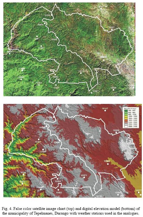
In this study, data from 41 weather stations were used (<a href="#t1">Table I</a>). These data were obtained through the Rapid Extractor of Weather Information (Extractor R&aacute;pido de Informaci&oacute;n Clim&aacute;tica&#150;ERIC) version 2 (IMTA, 2000). Since only four communities in this municipality have weather information, it was necessary to expand geographical coverage in order to have information analogous to the municipality's different climatic conditions (<a href="/img/revistas/atm/v21n1/a3f2.jpg" target="_blank">Fig. 2</a>). This meant that 37 new weather stations were included.</font></p>     <p align="center"><font face="verdana" size="2"><a name="t1"></a></font></p>     <p align="center"><font face="verdana" size="2"><img src="/img/revistas/atm/v21n1/a3t1.jpg"></font></p>     ]]></body>
<body><![CDATA[<p align="justify"><font face="verdana" size="2">&nbsp;</font></p>     <p align="justify"><font face="verdana" size="2"><i>2.3 Spatial estimation of temperature</i></font></p>     <p align="justify"><font face="verdana" size="2">The process of temperature estimation and the elaboration of isotherm maps is detailed as follows:</font></p>     <blockquote>       <p align="justify"><font face="verdana" size="2">1.&nbsp; Regionalization of the study area according to conditions that affect the temperature gradient.    <br>     These conditions are latitude, altitude, patterns of atmospheric circulation, local conditions, continental effects and characteristics of ocean currents, exposure to the sun in the regional mountainous systems, and air moisture content throughout the year (Ahrens, 2003).    <br>   For this particular study, the area was divided into two large portions: the western, or windward, and part of the high plateau of the mountainous region, and the leeward. The windward portion is affected by the humid winds of the Pacific Ocean blowing from June to October, known as the Mexican Monsoon (Douglas <i>et al., </i>1993; Stensrud <i>et al., </i>1995) and, in general, is more humid. The leeward portion comprises part of the high plateau, with less rainfall, and the valley zone which is the Tepehuanes River watershed, as well as the eastern side of the Sierra, which is drier (Monterroso&#150;Rivas and G&oacute;mez&#150;D&iacute;az, 2003) (<a href="/img/revistas/atm/v21n1/a3f2.jpg" target="_blank">Fig. 2</a>).</font></p>       <p align="justify"><font face="verdana" size="2">2.&nbsp; &nbsp;Selection of the meteorological stations with complete data set in the study area.    <br>   In the example shown here, the municipality was delimited using the regional digital elevation model and the four weather stations with reliable data were located within the municipal boundaries.</font></p>       <p align="justify"><font face="verdana" size="2">3.&nbsp; Expansion of the data collection area in order to have more data.    ]]></body>
<body><![CDATA[<br>   As the number of meteorological stations was not sufficient, it was necessary to increase coverage considering the characteristics that affect the temperature gradient defined in the initial delimitation of the different areas. The location and altitude of the meteorological stations were verified and corrections were introduced where necessary. Therefore, thirty&#150;seven weather stations were incorporated into the analysis.</font></p>       <p align="justify"><font face="verdana" size="2">4.&nbsp; Estimation of temperature on areas with complex landscape with simple regression equations. To estimate temperature within a landscape characterized by mountains, the simple or empirical method described by Ortiz&#150;Solorio (1989) was used. This method calculates regional lapse rates for each month and the annual mean, establishing simple regression equations between temperature and elevation.    <br>     Twenty&#150;four weather stations for the windward portion and twenty&#150;three for the leeward were chosen, while six stations from the high plateau were used for both zones (<a href="#t2">Table II</a>).    <br>   For each group of stations, a simple linear regression analysis was performed, obtaining twelve monthly models and one annual model. To determine whether the models were satisfactory, the statistical estimators of each were calculated: determination coefficient (R<sup>2</sup>), standard error, and probability of F distribution.</font></p>       <p align="center"><font face="verdana" size="2"><a name="t2"></a></font></p>       <p align="center"><font face="verdana" size="2"><img src="/img/revistas/atm/v21n1/a3t2.jpg"></font></p>       <p align="justify"><font face="verdana" size="2">5.&nbsp; &nbsp;Creating isotherm maps with the simpler regression equations.    <br>     The simple regression models were applied to each of the areas defined above. Thus, twelve monthly and one annual isotherm maps had to be constructed for each area. The maps were drawn using a digital topographic map and the site's digital elevation model, and detailed with the Arc View geographic information System (ESRI, 2004).    <br>   In each one of the areas in which the municipality was divided the simple regression models were incorporated for the monthly and annual reports to calculate the temperature corresponding to each interval of altitude above sea level. Temperatures calculated for the different altitudes within the municipality were arranged in accordance with one Celsius degree intervals. This procedure was applied separately to the windward and leeward portions. The isotherm maps were structured using an interval of one degree, starting from the lowest part of the territory to the highest. Polygons were established for each temperature interval, associated with meters above sea level of that temperature; values are expressed in whole numbers.</font></p>       <p align="justify"><font face="verdana" size="2">6.&nbsp; Isotherm maps for relatively flat areas.    ]]></body>
<body><![CDATA[<br>   In this study there were no flat areas, but in nearly flat areas with relatively small variations in altitude and with an acceptable number of meteorological stations, the monthly and annual isotherms maps are constructed with interpolation models such as kriging, or its variants, using Arc View Geographic Information System (ESRI, 2004).</font></p>       <p align="justify"><font face="verdana" size="2">7.&nbsp; &nbsp;Combination of the isotherm maps of the windward and leeward portions.    <br>     Monthly and annual isotherm maps of the different areas were combined, making adjustments in the areas where temperature range values differed. In the parts with lower temperature values, adjustments were made by using the same temperature intervals and reducing altitude intervals. In the parts where temperatures were higher, with the same temperature intervals, altitude intervals were increased until their values matched.    <br>   In this particular exercise, the monthly and annual isotherm maps of both portions were combined, making adjustments in the areas where temperature range values differed. The adjustments were made by increasing temperature ranges on the windward portion at small altitude differences, and on the leeward portion temperature ranges were decreased until their values matched. In this case, the largest difference between the temperature ranges in some parts of the junction zone was of two degrees.</font></p>       <p align="justify"><font face="verdana" size="2">8. Digital edition of monthly and annual mean temperature maps.    <br>   The monthly and annual maps of temperature are kept in digital format, assigning colors to each of the temperature ranges, based on the Instituto Nacional de Estad&iacute;stica, Geograf&iacute;a e Inform&aacute;tica (INEGI) proposal for the colors on its annual mean temperature maps of M&eacute;xico, at 1:1 000 000 scale (SPP, 1981).</font></p> </blockquote>     <p align="justify"><font face="verdana" size="2">&nbsp;</font></p>     <p align="justify"><font face="verdana" size="2"><i>2.4 Elaboration of precipitation maps</i></font></p>     <p align="justify"><font face="verdana" size="2"><i>2.4.1 Mean annual isohyet maps</i></font></p>     <p align="justify"><font face="verdana" size="2">The process of precipitation map construction is detailed as follow:</font></p>     ]]></body>
<body><![CDATA[<blockquote>       <p align="justify"><font face="verdana" size="2">1.&nbsp; &nbsp;Location of weather stations on a digital elevation model map.    <br>   The location of each of the weather stations must be identified geographically and the annual amount of rainfall reported.</font></p>       <p align="justify"><font face="verdana" size="2">2.&nbsp; &nbsp;Analysis of the relationship between the amount of rainfall and global and regional wind circulation systems.    <br>     For each weather station the amount of rainfall reported and its annual distribution must be analyzed, and a possible explanation must be given. To do this, it is necessary to have a general knowledge of the influence of the different meteorological systems throughout the year for each of the regions in which the amount of precipitation will be estimated.    <br>   In this study the data from two weather stations for rainfall distribution throughout the year in each portion (windward and leeward) were compared. One reported the highest annual amount of precipitation and the other the lowest value (<a href="/img/revistas/atm/v21n1/a3f3.jpg" target="_blank">Fig. 3a</a> for windward and <a href="/img/revistas/atm/v21n1/a3f3.jpg" target="_blank">3b</a> for leeward). It is clear that all the stations have very similar patterns of rainfall distribution. The rainy season is in summer, but there is also a small but significant winter rainfall. The summer rainfall over the windward slopes of the Sierra Madre Occidental and western high plateaus was associated with elements of the Monsoon of North America (Barlow <i>et al., </i>1998; Berbery, 2001; Higgins <i>et al., </i>2003), specifically, the component known as the Mexican Monsoon (Douglas <i>et al., </i>1993; Stensrud <i>et al., </i>1995; Berbery, 2001; Higgins <i>et al., </i>2003) (<a href="/img/revistas/atm/v21n1/a3f3.jpg" target="_blank">Fig. 3a</a>). In this system the prevailing winds blow mainly southwest to northeast. For the zone of valleys and the leeward part of the municipality, the rainy season was associated with the influence of moisture coming from the Gulf of M&eacute;xico (Tang and Reiter, 1984) as well as with the effect of the Mexican Monsoon (<a href="/img/revistas/atm/v21n1/a3f3.jpg" target="_blank">Fig. 3b</a>). In this system the prevailing winds blow east to west. The winter rainfall in both areas was associated to the impact of vortexes and cold fronts (Mosi&ntilde;o and Garc&iacute;a, 1974), where the prevailing winds blow from west to east.</font></p>       <p align="justify"><font face="verdana" size="2">3.&nbsp; &nbsp;Analysis of impacts of the climate&#150;modifying factors in the amount of rainfall.    <br>     The monthly amount of rainfall in each meteorological station must be analyzed, identifying the impact of the climate modifying factors, such as bodies of water, distance from the ocean, and orography including form of the mountain ridges, their orientation and aspect (Ahrens, 2003).    <br>     In this study, once the phenomena causing different amounts of precipitation were identified, the impact of orography of the areas where the weather stations were located was examined.    <br>   The amount of precipitation was explained as a result of the direction of moisture&#150;carrying winds throughout the year, and whether they arrive directly to those areas or bypass orographic units that may divert them or force them to ascend and lose moisture. Other factors also considered were the form and dimension of the mountain ridge, slope aspect, winds conducted through a canyon, the shadow effect of mountain barriers and other elements that contribute to explaining the magnitude of the rainfall reported in areas having weather information, and surrounding zones.</font></p>       ]]></body>
<body><![CDATA[<p align="justify"><font face="verdana" size="2">4. Search for relationships between the amount of rainfall and the color associated with vegetation on a false color satellite image.    <br>     All the meteorological stations were located in two different false color satellite images, one taken in the dry season and the other during the wet season. The meteorological stations must be situated in their place and the amount of annual rainfall reported. A relationship was sought between the amount of rainfall reported in each meteorological station and the false color associated with the natural vegetation and also with the position in the landscape, emphasizing the forms of the terrain and how they influence prevailing winds that carry rainfall&#150;producing moisture.    <br>   In this study the satellite image chart colors were reviewed to associate them with the vegetation and soil moisture so as to find a connection with the rainfall present in the sites having weather information. In general, a more intense color associated with vegetation was translated as a higher amount of rainfall. In this assumption, slope orientation has an enormous effect on soil moisture retention. At the latitude of the study site vegetation on the northern slope differs considerably from that of the southern slope even when the amount of rainfall is the same (<a href="#f4">Fig. 4</a>) as consequence of the amount of radiation received and its impact on availability of water to the vegetation (Ahrens, 2003).</font></p>       <p align="center"><font face="verdana" size="2"><a name="f4"></a></font></p>       <p align="center"><font face="verdana" size="2"><img src="/img/revistas/atm/v21n1/a3f4.jpg"></font></p>       <p align="justify"><font face="verdana" size="2">5.&nbsp; &nbsp;Search for analogies between sites with meteorological information and areas without meteorological stations.    <br>   These analogies were established by analyzing the prevailing wind direction and the modifying effect of this flow by the different elements of the landscape. Tentative values of mean annual precipitation were assigned to sites with similar land form conditions and similar location relative to the direction of prevailing winds. Values must be assigned matching the false color associated with condition of the natural vegetation.</font></p>       <p align="justify"><font face="verdana" size="2">6.&nbsp; &nbsp;Drawing the isohyet map on the digital elevation model.    <br>   Annual isohyets must be drawn manually on the digital elevation model based on the mean annual precipitation values assigned by analogy in the previous analysis and those values taken directly from weather stations. The process starts with the identification of the analogies that are easiest to locate; these, in general, correspond to the extreme values of precipitation. Intermediate isohyets are then drawn manually by joining the points defined after analyzing the effect of the different precipitation&#150;modifying factors and the local circulation of winds.</font></p>       <p align="justify"><font face="verdana" size="2">7.&nbsp; &nbsp;Edition of the mean annual isohyet map in digital format.    ]]></body>
<body><![CDATA[<br>   The manually&#150;drawn isohyet map of annual mean precipitation was reproduced digitally using the Arc View Geographic Information System (ESRI, 2004), generating areas defined by precipitation ranges.</font></p> </blockquote>     <p align="justify"><font face="verdana" size="2">&nbsp;</font></p>     <p align="justify"><font face="verdana" size="2"><i>2.4.2 Mean monthly isohyet maps</i></font></p>     <p align="justify"><font face="verdana" size="2">Monthly precipitation maps are based on the annual precipitation maps. The steps in this work are detailed as follows:</font></p>     <blockquote>       <p align="justify"><font face="verdana" size="2">1.&nbsp; Estimation of mean monthly values of precipitation for each annual range of rainfall.    <br>   For each of the areas, monthly precipitation data from the meteorological stations were previously subdivided according to the portion in which they are located (windward or leeward). The monthly data from the different stations located in a given area (defined by annual means) were averaged to obtain monthly precipitation values.</font></p>       <p align="justify"><font face="verdana" size="2">2.&nbsp; Estimation of mean monthly precipitation ranges.    <br>     The mean monthly precipitation ranges for each area defined by annual ranges were assigned according to the variation in mean precipitation reported for each month by the different groups of stations. Making sure that the monthly values add up to annual range be covered proportionally and that the adjacent sections of the two portions have the same precipitation range.    <br>   In the months of less precipitation the ranges established are narrow and in those months of heavy rains these ranges are considerably broader.</font></p>       ]]></body>
<body><![CDATA[<p align="justify"><font face="verdana" size="2">3.&nbsp; Estimation of proportional values of monthly precipitation.    <br>   The median of each monthly range was used as the estimation of monthly precipitation. It was verified that the sum of the monthly precipitation estimates was within the corresponding annual mean precipitation range.</font></p>       <p align="justify"><font face="verdana" size="2">4.&nbsp; Correlation of mean monthly precipitation estimates and averages reported by the meteorological stations.    <br>   For each annual precipitation range a simple linear regression analysis was performed between the mean precipitation calculated from data obtained from the groups of weather stations and the median values of the monthly ranges. To determine whether the models were satisfactory, their statistics estimators &#150;coefficient of determination (R<sub>2</sub>), standard error, and the probability of F distribution&#150; were calculated for each linear regression model.</font></p>       <p align="justify"><font face="verdana" size="2">5.&nbsp; Edition of the mean annual isohyet map in digital format.    <br>   Monthly precipitation maps were constructed using the areas delimiting annual average precipitation ranges using the Arc View Geographic Information System (ESRI, 2004).</font></p> </blockquote>     <p align="justify"><font face="verdana" size="2">&nbsp;</font></p>     <p align="justify"><font face="verdana" size="2"><b>3. Results and discussion</b></font></p>     <p align="justify"><font face="verdana" size="2"><i>3.1 Isotherm maps</i></font></p>     <p align="justify"><font face="verdana" size="2"><a href="#t2">Tables II</a> and <a href="#t3">III</a> show the results of regional temperature models with statistical diagnoses.</font></p>     ]]></body>
<body><![CDATA[<p align="center"><font face="verdana" size="2"><a name="t3"></a></font></p>     <p align="center"><font face="verdana" size="2"><img src="/img/revistas/atm/v21n1/a3t3.jpg"></font></p>     <p align="justify"><font face="verdana" size="2">There was a clear difference in the study area temperature ranges between the extreme values on the leeward portion (<a href="#t3">Table III</a>) as a consequence of less moisture in the air, and the smaller variations on the windward portion (<a href="#t3">Table III</a>) at the same heights (Arhens, 2003).</font></p>     <p align="justify"><font face="verdana" size="2">In both cases the determination coefficients (R<sup>2</sup>) were satisfactory, above 0.9 on the windward and 0.8 on the leeward. The standard errors on the windward portion were in all cases below 1 &deg;C (0.43 to 0.70 &deg;C); on the leeward portion these values were higher, ranging from 0.83 to 1.47 &deg;C. In both cases the calculated F distribution was considerably higher than F from tables, with a 0.001 level of significance. Forthe windward portion, F from tables was 14.4, and forthe leeward it was 15.1, which shows that the regression coefficients in the models representing elevation lapse rates of temperature variation are highly significant. The windward regressions are better defined and this is probably due to the broad elevation range used.</font></p>     <p align="justify"><font face="verdana" size="2">For the estimation of monthly and annual mean temperatures in areas of complex relief and scarce weather stations it is critical to establish a relationship between elevation and temperature variation ranges (Hutchinson, 1987). Moreover, interpolation methods must include objective techniques together with statistical diagnoses that have previously quantified predicted errors (Mackey <i>et al., </i>1996).</font></p>     <p align="justify"><font face="verdana" size="2">According to literature, in the construction of monthly and annual models it is necessary to delimit areas with similar temperature elevation lapse rates in each region, considering such factors that might affect such lapse rates, as the following:</font></p>     <blockquote>       <p align="justify"><font face="verdana" size="2">1.&nbsp; The modifying effect of water bodies on temperature changes (Arhens, 2003).</font></p>       <p align="justify"><font face="verdana" size="2">2.&nbsp; Moisture conditions of the area, which are generally associated with the effect of mountain ridges on rainfall distribution.    <br>   Thus, attention is given to the effect of air moisture on the vertical temperature lapse rate, which is lower in humid zones (Stull, 2000; Arhens, 2003).</font></p>       ]]></body>
<body><![CDATA[<p align="justify"><font face="verdana" size="2">3.&nbsp; The orientation of mountain ridges, which separates the effect of incoming solar radiation on temperature (Aguado and Burt, 2001); the northern slope in subtropical regions of M&eacute;xico tends to be cooler.    <br>     The moisture condition factor of this exercise was taken into account due to the specific conditions of the area under study.    <br>     There are considerable differences between the windward and leeward portions in terms of annual and monthly temperature lapse trends as altitude increases. On the leeward slope temperature lapse rates were higher than on the windward. At similar altitudes, there are considerable differences in mean temperature between the two portions, especially at lower elevations; however, as elevation increases, the temperature ranges become more similar. This is due to the cooling trend of humid air rising from the windward portion of the Sierra, which leaves part of its moisture in this zone and releases latent heat in the condensation of water vapor to then descend as dry air towards the region of valleys (Ahrens, 2003). The release of latent heat of the water vapor on the windward side warms the air, and the cooling rate of ascending air range diminishes. The trends in rapid temperature change with changes in altitude on the leeward portion can be explained by the dry adiabatic lapse rate that can be up to 1 &deg;C for each 100 m (Aguado and Burt, 2001) because the air is drier than on the windward portion, especially during the hottest months. The elevation range of the weather stations on the leeward portion was between 1660 to 2690 m and, due to the high temperature lapse rate in each model, the hypothetical mean monthly values at sea level of the hottest and also driest months were very high (40.55 and 41.32 &deg;C for May and June, respectively).    <br>     <a href="/img/revistas/atm/v21n1/a3f5.jpg" target="_blank">Figure 5</a> shows the maps of monthly mean temperatures in January (5b) and May (5c) and <a href="/img/revistas/atm/v21n1/a3f5.jpg" target="_blank">Figure 5a</a> shows the map of annual mean temperature, after combining the windward and leeward portions. The finest detail in the different temperature range areas is clear as a result of the use of the digital elevation model.</font></p> </blockquote>     <p align="justify"><font face="verdana" size="2">&nbsp;</font></p>     <p align="justify"><font face="verdana" size="2"><i>3.2 Isohyet maps</i></font></p>     <p align="justify"><font face="verdana" size="2"><a href="/img/revistas/atm/v21n1/a3f6.jpg" target="_blank">Figure 6</a> clearly shows the influence of moist winds from the Pacific Ocean on mean precipitation, especially on the windward portion of the Sierra, which is associated with the Mexican Monsoon (Douglas <i>et al., </i>1993, Stensrud, <i>et al., </i>1995; Berbery, 2001; Higgins <i>et al., </i>2003), and the orographic rainshadow in the region of valleys. On the leeward portion of the Sierra it is possible to detect the influence of winds with a lower content of moisture which travels at a greater height from the Gulf of M&eacute;xico (Barlow <i>et al., </i>1998); these winds are usually associated with lower amount of precipitation.</font></p>     <p align="justify"><font face="verdana" size="2">The relation between precipitation measured in weather stations and elevation can vary from one mountain to another since rainfalls are influenced by such factors as the dimension of the mountain barrier, slope differences and land form, mountain ridges orientation, their position in relation to the prevailing winds, whether winds come directly or have passed by other mountain systems, which side of the mountain winds rise or descend, whether they have been diverted or conducted through a canyon (Mosi&ntilde;o and Garcia, 1974). All this makes it difficult to establish reasonable relationships between elevation and precipitation since there are few stations in the region registering the differences associated with the factors mentioned above (Daly <i>et al., </i>1994).</font></p>     <p align="justify"><font face="verdana" size="2">Due to the specific conditions of the study area &#150;similar to a large part of the mountain regions in M&eacute;xico where the lack of meteorological information is frequent&#150; the proposed method for the elaboration of isohyet maps can be classified as graphic, in which an analysis was made of the factors influencing the distribution of precipitation and of the information on the atmosphere's local circulation throughout the year.</font></p>     <p align="justify"><font face="verdana" size="2">Monthly ranges were set so that the mean precipitation estimated would fall within annual ranges; this was the case for most of the situations. There were few cases in which this did not occur due to the criterion that the larger the amount of annual precipitation, the larger the amount of monthly precipitation must be.</font></p>     ]]></body>
<body><![CDATA[<p align="justify"><font face="verdana" size="2">The estimated values of monthly precipitation for each annual range were the median of the interval. The sum of all the estimated monthly mean precipitations was within the expected annual range.</font></p>     <p align="justify"><font face="verdana" size="2"><a href="#t4">Table IV</a> shows the linear regression models between the statistical parameters on the windward portion and <a href="#t5">Table V</a> presents those for the leeward. In both cases R<sup>2</sup> values were satisfactory, above 0.96, most of them between 0.98 and 0.99. The standard errors were between 1.4 to 6.1 mm and from 1.0 to 7.0 mm of monthly rainfall for the windward and leeward portion, respectively. These are acceptable, based on the values of monthly rainfall reported in the weather stations. The F distribution calculated was considerably higher than F from tables with a 0.001 level of significance. For the different monthly levels, F from tables was 21.0 for the general model; 11.7 for the windward model and 11.8 for the leeward. This shows that the regression coefficients in models representing the relationship between the average precipitation calculated for the different weather stations and the value of precipitation estimated by the procedure indicated in this paper of the different groups of stations (by annual precipitation ranges) are highly significant.</font></p>     <p align="center"><font face="verdana" size="2"><a name="t4"></a></font></p>     <p align="center"><font face="verdana" size="2"><img src="/img/revistas/atm/v21n1/a3t4.jpg"></font></p>     <p align="center"><font face="verdana" size="2"><a name="t5"></a></font></p>     <p align="center"><font face="verdana" size="2"><img src="/img/revistas/atm/v21n1/a3t5.jpg"></font></p>     <p align="justify"><font face="verdana" size="2">The monthly mean precipitation maps elaborated in accordance with the ranges established are presented in <a href="/img/revistas/atm/v21n1/a3f6.jpg" target="_blank">Figure 6b and c</a>. They also show the great influence of orography on the distribution of precipitation throughout the year.</font></p>     <p align="justify"><font face="verdana" size="2">&nbsp;</font></p>     <p align="justify"><font face="verdana" size="2"><b>4. Conclusions</b></font></p>     <p align="justify"><font face="verdana" size="2">The methodology proposed to estimate temperature and monthly and annual mean precipitation in areas of complex relief and little meteorological information served to draw detailed maps of these variables.</font></p>     ]]></body>
<body><![CDATA[<p align="justify"><font face="verdana" size="2">In the case of temperature, the models estimated by applying the simple method, previously subdividing the zone according to moisture conditions, resulted in highly satisfactory statistical estimators; thus, it can be concluded that the methodology fulfills its purpose.</font></p>     <p align="justify"><font face="verdana" size="2">The application of the Arc View Geographical Information System (ESRI, 2004) provides a clear image of the relation between the location elevation and temperature.</font></p>     <p align="justify"><font face="verdana" size="2">The estimation procedure for precipitation, based on the graphic method, produces detailed maps of this variable, although it requires considerable knowledge of local circulation of the atmosphere in the region throughout the year and also of the effect of orography on the processes causing precipitation. For the analogies established to enable the estimations, the different reports given by the weather stations, the specific conditions in which these stations are located and the vegetation reflectance shown in the false color satellite images (satellite image chart) through differences in colors are all essential.</font></p>     <p align="justify"><font face="verdana" size="2">The monthly precipitation estimated for each of the annual ranges established correlates highly with the mean precipitation obtained as averages from the stations grouped within each annual precipitation range on both portions of the Sierra.</font></p>     <p align="justify"><font face="verdana" size="2">This technique has great potential in the drawing of maps of monthly and annual mean temperature and precipitation at local and regional level in areas with little meteorological information and complex relief.</font></p>     <p align="justify"><font face="verdana" size="2">&nbsp;</font></p>     <p align="justify"><font face="verdana" size="2"><b>References</b></font></p>     <!-- ref --><p align="justify"><font face="verdana" size="2">Ahrens C. D., 2003. <i>Meteorology today: an introduction to weather, climate, and the environment. </i>7th Ed. Brooks Cole. Pacific Grove, CA, USA, 594 pp.</font>&nbsp;&nbsp;&nbsp;&nbsp;&nbsp;&nbsp;&nbsp;&nbsp;[&#160;<a href="javascript:void(0);" onclick="javascript: window.open('/scielo.php?script=sci_nlinks&ref=1266555&pid=S0187-6236200800010000300001&lng=','','width=640,height=500,resizable=yes,scrollbars=1,menubar=yes,');">Links</a>&#160;]<!-- end-ref --><!-- ref --><p align="justify"><font face="verdana" size="2">Aguado E. and J. E. Burt, 2001. <i>Understanding weather and climate. </i>2nd ed. Prentice Hall, Upper Saddle River, New Jersey, USA, 505 pp.</font>&nbsp;&nbsp;&nbsp;&nbsp;&nbsp;&nbsp;&nbsp;&nbsp;[&#160;<a href="javascript:void(0);" onclick="javascript: window.open('/scielo.php?script=sci_nlinks&ref=1266556&pid=S0187-6236200800010000300002&lng=','','width=640,height=500,resizable=yes,scrollbars=1,menubar=yes,');">Links</a>&#160;]<!-- end-ref --><!-- ref --><p align="justify"><font face="verdana" size="2">Barlow M., S. Nigam and E. H. Berbery, 1998. Evolution of the North American monsoon system. <i>J. Climate. </i><b>11, </b>2238&#150;2257.</font>&nbsp;&nbsp;&nbsp;&nbsp;&nbsp;&nbsp;&nbsp;&nbsp;[&#160;<a href="javascript:void(0);" onclick="javascript: window.open('/scielo.php?script=sci_nlinks&ref=1266557&pid=S0187-6236200800010000300003&lng=','','width=640,height=500,resizable=yes,scrollbars=1,menubar=yes,');">Links</a>&#160;]<!-- end-ref --><!-- ref --><p align="justify"><font face="verdana" size="2">Barry R. G., 1992. <i>Montain weather and climate. </i>2nd Ed. Routledge, London, 402 pp.</font>&nbsp;&nbsp;&nbsp;&nbsp;&nbsp;&nbsp;&nbsp;&nbsp;[&#160;<a href="javascript:void(0);" onclick="javascript: window.open('/scielo.php?script=sci_nlinks&ref=1266558&pid=S0187-6236200800010000300004&lng=','','width=640,height=500,resizable=yes,scrollbars=1,menubar=yes,');">Links</a>&#160;]<!-- end-ref --><!-- ref --><p align="justify"><font face="verdana" size="2">Berbery E. H., 2001. Mesoscale moisture analysis of the North American monsoon. <i>J. Climate. </i><b>14</b>, 121&#150;137.</font>&nbsp;&nbsp;&nbsp;&nbsp;&nbsp;&nbsp;&nbsp;&nbsp;[&#160;<a href="javascript:void(0);" onclick="javascript: window.open('/scielo.php?script=sci_nlinks&ref=1266559&pid=S0187-6236200800010000300005&lng=','','width=640,height=500,resizable=yes,scrollbars=1,menubar=yes,');">Links</a>&#160;]<!-- end-ref --><!-- ref --><p align="justify"><font face="verdana" size="2">Burns J. I., 1953. Small&#150;scale topographic effects on precipitation distribution in San Dimas Experimental Forest. <i>Trans. Am. Geophys. Union </i><b>34</b>, 761&#150;768.</font>&nbsp;&nbsp;&nbsp;&nbsp;&nbsp;&nbsp;&nbsp;&nbsp;[&#160;<a href="javascript:void(0);" onclick="javascript: window.open('/scielo.php?script=sci_nlinks&ref=1266560&pid=S0187-6236200800010000300006&lng=','','width=640,height=500,resizable=yes,scrollbars=1,menubar=yes,');">Links</a>&#160;]<!-- end-ref --><!-- ref --><p align="justify"><font face="verdana" size="2">Creutin J. D. and C. Obled, 1982. Objective analysis and mapping techniques for rainfall fields: an objective comparison. <i>Water Resour. Res. </i><b>18</b>, 413&#150;431.</font>&nbsp;&nbsp;&nbsp;&nbsp;&nbsp;&nbsp;&nbsp;&nbsp;[&#160;<a href="javascript:void(0);" onclick="javascript: window.open('/scielo.php?script=sci_nlinks&ref=1266561&pid=S0187-6236200800010000300007&lng=','','width=640,height=500,resizable=yes,scrollbars=1,menubar=yes,');">Links</a>&#160;]<!-- end-ref --><!-- ref --><p align="justify"><font face="verdana" size="2">Daly C., R. P. Nielson and D. L. Phillips, 1994. A statistical&#150;topographic model for mapping climatological precipitation over mountainous terrain. <i>J. Appl. Meteorol. </i><b>33</b>, 140&#150;158.</font>&nbsp;&nbsp;&nbsp;&nbsp;&nbsp;&nbsp;&nbsp;&nbsp;[&#160;<a href="javascript:void(0);" onclick="javascript: window.open('/scielo.php?script=sci_nlinks&ref=1266562&pid=S0187-6236200800010000300008&lng=','','width=640,height=500,resizable=yes,scrollbars=1,menubar=yes,');">Links</a>&#160;]<!-- end-ref --><!-- ref --><p align="justify"><font face="verdana" size="2">Dingman S. L., D. M. Seely&#150;Reynolds and R. C. Reynolds III, 1988. Application of kriging to estimating mean annual precipitation in a region of orographic influence. <i>Water Resources B. </i><b>24</b>, 329&#150;339.</font>&nbsp;&nbsp;&nbsp;&nbsp;&nbsp;&nbsp;&nbsp;&nbsp;[&#160;<a href="javascript:void(0);" onclick="javascript: window.open('/scielo.php?script=sci_nlinks&ref=1266563&pid=S0187-6236200800010000300009&lng=','','width=640,height=500,resizable=yes,scrollbars=1,menubar=yes,');">Links</a>&#160;]<!-- end-ref --><!-- ref --><p align="justify"><font face="verdana" size="2">Douglas M. W., R. A. Maddox, K. Howard and S. Reyes, 1993. The Mexican monsoon. <i>J. Climate </i><b>6</b>, 1665&#150;1667.</font>&nbsp;&nbsp;&nbsp;&nbsp;&nbsp;&nbsp;&nbsp;&nbsp;[&#160;<a href="javascript:void(0);" onclick="javascript: window.open('/scielo.php?script=sci_nlinks&ref=1266564&pid=S0187-6236200800010000300010&lng=','','width=640,height=500,resizable=yes,scrollbars=1,menubar=yes,');">Links</a>&#160;]<!-- end-ref --><!-- ref --><p align="justify"><font face="verdana" size="2">ESRI, 1996. Environmental Systems Research Institute, Inc., 380 New York Street. Redlands, CA. 92373 USA.</font>&nbsp;&nbsp;&nbsp;&nbsp;&nbsp;&nbsp;&nbsp;&nbsp;[&#160;<a href="javascript:void(0);" onclick="javascript: window.open('/scielo.php?script=sci_nlinks&ref=1266565&pid=S0187-6236200800010000300011&lng=','','width=640,height=500,resizable=yes,scrollbars=1,menubar=yes,');">Links</a>&#160;]<!-- end-ref --><!-- ref --><p align="justify"><font face="verdana" size="2">Gandin L. S., 1963. Objective analysis of meteorological fields. Israel Programme for Scientific Translation (translated from Russian, 1965), Jerusalem.</font>&nbsp;&nbsp;&nbsp;&nbsp;&nbsp;&nbsp;&nbsp;&nbsp;[&#160;<a href="javascript:void(0);" onclick="javascript: window.open('/scielo.php?script=sci_nlinks&ref=1266566&pid=S0187-6236200800010000300012&lng=','','width=640,height=500,resizable=yes,scrollbars=1,menubar=yes,');">Links</a>&#160;]<!-- end-ref --><!-- ref --><p align="justify"><font face="verdana" size="2">Garc&iacute;a Benavides J., 1979. Estructura metodol&oacute;gica para la caracterizaci&oacute;n agroecol&oacute;gica de &aacute;reas por procedimientos cuantitativos de an&aacute;lisis y su posterior zonificaci&oacute;n. Tesis de Doctor en Ciencias. Colegio de Posgraduados, Chapingo, M&eacute;xico, 401 pp.</font>&nbsp;&nbsp;&nbsp;&nbsp;&nbsp;&nbsp;&nbsp;&nbsp;[&#160;<a href="javascript:void(0);" onclick="javascript: window.open('/scielo.php?script=sci_nlinks&ref=1266567&pid=S0187-6236200800010000300013&lng=','','width=640,height=500,resizable=yes,scrollbars=1,menubar=yes,');">Links</a>&#160;]<!-- end-ref --><!-- ref --><p align="justify"><font face="verdana" size="2">Higgins R. W., A. Douglas, A. Hahmann, E. H. Berbery, D. Gutzler, J. Shuttleworth, D. Stensrud, J. Amador, R. Carbone, M. Cortez, M. Douglas, R. Lobato, J. Meitin, C. Ropelewski, J. Schemm, S. Schubert and C. Zhang, 2003. Progress in Pan American CLIVAR research: The North American Monsoon System. <i>Atm&oacute;sfera </i><b>16</b>, 29&#150;65.</font>&nbsp;&nbsp;&nbsp;&nbsp;&nbsp;&nbsp;&nbsp;&nbsp;[&#160;<a href="javascript:void(0);" onclick="javascript: window.open('/scielo.php?script=sci_nlinks&ref=1266568&pid=S0187-6236200800010000300014&lng=','','width=640,height=500,resizable=yes,scrollbars=1,menubar=yes,');">Links</a>&#160;]<!-- end-ref --><!-- ref --><p align="justify"><font face="verdana" size="2">Houghton J. G., 1979. A model for orographic precipitation in the North&#150;Central Great Basin. <i>Mon. Wea. Rev. </i><b>107</b>, 1462&#150;1475.</font>&nbsp;&nbsp;&nbsp;&nbsp;&nbsp;&nbsp;&nbsp;&nbsp;[&#160;<a href="javascript:void(0);" onclick="javascript: window.open('/scielo.php?script=sci_nlinks&ref=1266569&pid=S0187-6236200800010000300015&lng=','','width=640,height=500,resizable=yes,scrollbars=1,menubar=yes,');">Links</a>&#160;]<!-- end-ref --><!-- ref --><p align="justify"><font face="verdana" size="2">Houghton J. T., L. G. Meiro Filho, B. A. Callander and N. Harris 1996. <i>Climate Change 1995: The science of climate change. </i>(A. Kattenburg and K. Maskell, Eds.). Cambridge University Press, Cambridge, 584 pp.</font>&nbsp;&nbsp;&nbsp;&nbsp;&nbsp;&nbsp;&nbsp;&nbsp;[&#160;<a href="javascript:void(0);" onclick="javascript: window.open('/scielo.php?script=sci_nlinks&ref=1266570&pid=S0187-6236200800010000300016&lng=','','width=640,height=500,resizable=yes,scrollbars=1,menubar=yes,');">Links</a>&#160;]<!-- end-ref --><!-- ref --><p align="justify"><font face="verdana" size="2">Hutchinson M. F., 1987. Methods of generation of weather sequences. In: <i>Agricultural environments: Characterizaction, classification and mapping. A. </i>H. Bunting, Ed.), CAB International, Wallingford, UK, 335 pp.</font>&nbsp;&nbsp;&nbsp;&nbsp;&nbsp;&nbsp;&nbsp;&nbsp;[&#160;<a href="javascript:void(0);" onclick="javascript: window.open('/scielo.php?script=sci_nlinks&ref=1266571&pid=S0187-6236200800010000300017&lng=','','width=640,height=500,resizable=yes,scrollbars=1,menubar=yes,');">Links</a>&#160;]<!-- end-ref --><!-- ref --><p align="justify"><font face="verdana" size="2">Hutchinson M. F. and R. J. Bischof, 1983. A new method of estimating mean seasonal and annual rainfall forthe Hunter Valley, New South Wales. <i>Aust. Meteorol. Mag. </i><b>31</b>, 179&#150;184.</font>&nbsp;&nbsp;&nbsp;&nbsp;&nbsp;&nbsp;&nbsp;&nbsp;[&#160;<a href="javascript:void(0);" onclick="javascript: window.open('/scielo.php?script=sci_nlinks&ref=1266572&pid=S0187-6236200800010000300018&lng=','','width=640,height=500,resizable=yes,scrollbars=1,menubar=yes,');">Links</a>&#160;]<!-- end-ref --><!-- ref --><p align="justify"><font face="verdana" size="2">IMTA, 2000. Extractor R&aacute;pido de Informaci&oacute;n Climatol&oacute;gica. Instituto Mexicano de Tecnolog&iacute;a del Agua, ERIC CD&#150;ROM. Cuernavaca, Mor. M&eacute;xico.</font>&nbsp;&nbsp;&nbsp;&nbsp;&nbsp;&nbsp;&nbsp;&nbsp;[&#160;<a href="javascript:void(0);" onclick="javascript: window.open('/scielo.php?script=sci_nlinks&ref=1266573&pid=S0187-6236200800010000300019&lng=','','width=640,height=500,resizable=yes,scrollbars=1,menubar=yes,');">Links</a>&#160;]<!-- end-ref --><!-- ref --><p align="justify"><font face="verdana" size="2">INEGI, 1993. Espaciomapas Hojas G13 &#150; 4, G13 &#150; 5, G13 &#150; 7, G13 &#150; 8, G13 &#150; 10 G13 &#150;11. Instituto Nacional de Estad&iacute;stica, Geograf&iacute;a e Inform&aacute;tica. Direcci&oacute;n General de Geograf&iacute;a. Aguascalientes, M&eacute;xico.</font>&nbsp;&nbsp;&nbsp;&nbsp;&nbsp;&nbsp;&nbsp;&nbsp;[&#160;<a href="javascript:void(0);" onclick="javascript: window.open('/scielo.php?script=sci_nlinks&ref=1266574&pid=S0187-6236200800010000300020&lng=','','width=640,height=500,resizable=yes,scrollbars=1,menubar=yes,');">Links</a>&#160;]<!-- end-ref --><!-- ref --><p align="justify"><font face="verdana" size="2">IPCC, 2001. Climate Change 2001: Synthesis report. Contribution of Working Groups I, II, and III to the Third Assessment Report of the Intergovernmental Panel on Climate Change. Cambridge University Press, New York, 33 pp.</font>&nbsp;&nbsp;&nbsp;&nbsp;&nbsp;&nbsp;&nbsp;&nbsp;[&#160;<a href="javascript:void(0);" onclick="javascript: window.open('/scielo.php?script=sci_nlinks&ref=1266575&pid=S0187-6236200800010000300021&lng=','','width=640,height=500,resizable=yes,scrollbars=1,menubar=yes,');">Links</a>&#160;]<!-- end-ref --><!-- ref --><p align="justify"><font face="verdana" size="2">Kleinbaum D. G., L. L. Kupper and K. E. Muller, 1988. Applied regression analysis and other multivariable methods. 2nd Edition. PWS&#150;Kent Publishing, Boston, MA, 718 pp.</font>&nbsp;&nbsp;&nbsp;&nbsp;&nbsp;&nbsp;&nbsp;&nbsp;[&#160;<a href="javascript:void(0);" onclick="javascript: window.open('/scielo.php?script=sci_nlinks&ref=1266576&pid=S0187-6236200800010000300022&lng=','','width=640,height=500,resizable=yes,scrollbars=1,menubar=yes,');">Links</a>&#160;]<!-- end-ref --><!-- ref --><p align="justify"><font face="verdana" size="2">Lookingbill T. R. and D. L. Urban, 2003. Spatial estimation of air temperature differences for landscape&#150;scale studies in montane environments. <i>Agr. For. Meteorol. </i><b>114</b>, 141&#150;151.</font>&nbsp;&nbsp;&nbsp;&nbsp;&nbsp;&nbsp;&nbsp;&nbsp;[&#160;<a href="javascript:void(0);" onclick="javascript: window.open('/scielo.php?script=sci_nlinks&ref=1266577&pid=S0187-6236200800010000300023&lng=','','width=640,height=500,resizable=yes,scrollbars=1,menubar=yes,');">Links</a>&#160;]<!-- end-ref --><!-- ref --><p align="justify"><font face="verdana" size="2">MacIver D. C. and R. D. Whitewood, 1992. Forest climates of Ontario. Part I. Bioclimate profiles 1968&#150;1988. Environment Canada, Atmospheric Environment Service, Ontario Ministry of Natural Resources, Toronto. </font>&nbsp;&nbsp;&nbsp;&nbsp;&nbsp;&nbsp;&nbsp;&nbsp;[&#160;<a href="javascript:void(0);" onclick="javascript: window.open('/scielo.php?script=sci_nlinks&ref=1266578&pid=S0187-6236200800010000300024&lng=','','width=640,height=500,resizable=yes,scrollbars=1,menubar=yes,');">Links</a>&#160;]<!-- end-ref --><!-- ref --><p align="justify"><font face="verdana" size="2">Mckey B. G., D. W. Mckenney, Y. Q. Yang, J. P. McMahon and M. F. Hutchinson, 1996. Site regions revisited: a climatic analysis of Hill's site regions for the province of Ontario using a parametric method. <i>Can. J. For. Res. </i><b>26</b>, 333&#150;354.</font>&nbsp;&nbsp;&nbsp;&nbsp;&nbsp;&nbsp;&nbsp;&nbsp;[&#160;<a href="javascript:void(0);" onclick="javascript: window.open('/scielo.php?script=sci_nlinks&ref=1266579&pid=S0187-6236200800010000300025&lng=','','width=640,height=500,resizable=yes,scrollbars=1,menubar=yes,');">Links</a>&#160;]<!-- end-ref --><!-- ref --><p align="justify"><font face="verdana" size="2">Monterroso&#150;Rivas A. I and J. D. G&oacute;mez&#150;D&iacute;az, 2003. <i>Escenarios climatol&oacute;gicos de la Rep&uacute;blica Mexicana ante el cambio clim&aacute;tico. </i>Comisi&oacute;n Nacional de las Zonas &Aacute;ridas y Universidad Aut&oacute;noma Chapingo. Chapingo, M&eacute;x. 170 pp.</font>&nbsp;&nbsp;&nbsp;&nbsp;&nbsp;&nbsp;&nbsp;&nbsp;[&#160;<a href="javascript:void(0);" onclick="javascript: window.open('/scielo.php?script=sci_nlinks&ref=1266580&pid=S0187-6236200800010000300026&lng=','','width=640,height=500,resizable=yes,scrollbars=1,menubar=yes,');">Links</a>&#160;]<!-- end-ref --><!-- ref --><p align="justify"><font face="verdana" size="2">Mosi&ntilde;o P. A. and E. Garc&iacute;a, 1974. The climate of M&eacute;xico. In: <i>World Survey of Climatology. </i>(R.A. Bryson and F. K. Hare, Eds.) Vol. II, Climates of North America, Elsevier, 373&#150;404.</font>&nbsp;&nbsp;&nbsp;&nbsp;&nbsp;&nbsp;&nbsp;&nbsp;[&#160;<a href="javascript:void(0);" onclick="javascript: window.open('/scielo.php?script=sci_nlinks&ref=1266581&pid=S0187-6236200800010000300027&lng=','','width=640,height=500,resizable=yes,scrollbars=1,menubar=yes,');">Links</a>&#160;]<!-- end-ref --><!-- ref --><p align="justify"><font face="verdana" size="2">Nalder I. A. and R. W. Wein, 1998. Spatial interpolation of climatic normals: test of a new method in the Canadian boreal forest. <i>Agr. For. Meteorol. </i><b>9</b>, 211&#150;225</font>&nbsp;&nbsp;&nbsp;&nbsp;&nbsp;&nbsp;&nbsp;&nbsp;[&#160;<a href="javascript:void(0);" onclick="javascript: window.open('/scielo.php?script=sci_nlinks&ref=1266582&pid=S0187-6236200800010000300028&lng=','','width=640,height=500,resizable=yes,scrollbars=1,menubar=yes,');">Links</a>&#160;]<!-- end-ref --><!-- ref --><p align="justify"><font face="verdana" size="2">Ortiz Solorio C. A., 1987. Elementos de agrometeorolog&iacute;a cuantitativa: con aplicaciones en la Rep&uacute;blica Mexicana. Departamento de Suelos, Universidad Aut&oacute;noma Chapingo, Chapingo, M&eacute;xico, 327 pp.</font>&nbsp;&nbsp;&nbsp;&nbsp;&nbsp;&nbsp;&nbsp;&nbsp;[&#160;<a href="javascript:void(0);" onclick="javascript: window.open('/scielo.php?script=sci_nlinks&ref=1266583&pid=S0187-6236200800010000300029&lng=','','width=640,height=500,resizable=yes,scrollbars=1,menubar=yes,');">Links</a>&#160;]<!-- end-ref --><!-- ref --><p align="justify"><font face="verdana" size="2">Peck E. L. and M. J. Brown, 1962. An approach to the development of isohyetal maps for mountainous areas. <i>J. Geophys. Res. </i><b>67</b>, 681&#150;694.</font>&nbsp;&nbsp;&nbsp;&nbsp;&nbsp;&nbsp;&nbsp;&nbsp;[&#160;<a href="javascript:void(0);" onclick="javascript: window.open('/scielo.php?script=sci_nlinks&ref=1266584&pid=S0187-6236200800010000300030&lng=','','width=640,height=500,resizable=yes,scrollbars=1,menubar=yes,');">Links</a>&#160;]<!-- end-ref --><!-- ref --><p align="justify"><font face="verdana" size="2">Phillips D. L., J. Dolph and D. Marks, 1992. A comparison of geostatistical procedures for spatial analysis of precipitation in mountainous terrain. <i>Agric. For. Meteorol. </i><b>58</b>, 119&#150;141.</font>&nbsp;&nbsp;&nbsp;&nbsp;&nbsp;&nbsp;&nbsp;&nbsp;[&#160;<a href="javascript:void(0);" onclick="javascript: window.open('/scielo.php?script=sci_nlinks&ref=1266585&pid=S0187-6236200800010000300031&lng=','','width=640,height=500,resizable=yes,scrollbars=1,menubar=yes,');">Links</a>&#160;]<!-- end-ref --><!-- ref --><p align="justify"><font face="verdana" size="2">Price D. T., D. W. McKenney, I. A. Nalder, M. F. Hutchinson and J. L. Kesteven, 2000. A comparison of two statistical methods for spatial interpolation of Canadian monthly climate data. <i>Agr. For. Meteorol. </i><b>101</b>, 81&#150;94.</font>&nbsp;&nbsp;&nbsp;&nbsp;&nbsp;&nbsp;&nbsp;&nbsp;[&#160;<a href="javascript:void(0);" onclick="javascript: window.open('/scielo.php?script=sci_nlinks&ref=1266586&pid=S0187-6236200800010000300032&lng=','','width=640,height=500,resizable=yes,scrollbars=1,menubar=yes,');">Links</a>&#160;]<!-- end-ref --><!-- ref --><p align="justify"><font face="verdana" size="2">Reed W. G. and J. B. Kince, 1917. The preparation of precipitation charts. <i>Mon. Wea. Rev. </i><b>45</b>, 233&#150;235.</font>&nbsp;&nbsp;&nbsp;&nbsp;&nbsp;&nbsp;&nbsp;&nbsp;[&#160;<a href="javascript:void(0);" onclick="javascript: window.open('/scielo.php?script=sci_nlinks&ref=1266587&pid=S0187-6236200800010000300033&lng=','','width=640,height=500,resizable=yes,scrollbars=1,menubar=yes,');">Links</a>&#160;]<!-- end-ref --><!-- ref --><p align="justify"><font face="verdana" size="2">Schermerhorn V. P., 1967. Relations between topography and annual precipitation in western Oregon and Washington. <i>Water Res. Res. </i><b>3</b>, 707&#150;711.</font>&nbsp;&nbsp;&nbsp;&nbsp;&nbsp;&nbsp;&nbsp;&nbsp;[&#160;<a href="javascript:void(0);" onclick="javascript: window.open('/scielo.php?script=sci_nlinks&ref=1266588&pid=S0187-6236200800010000300034&lng=','','width=640,height=500,resizable=yes,scrollbars=1,menubar=yes,');">Links</a>&#160;]<!-- end-ref --><!-- ref --><p align="justify"><font face="verdana" size="2">SPP, 1981. Cartas de temperatura media anual de la Rep&uacute;blica Mexicana escala 1: 1000000. Direcci&oacute;n General de Geograf&iacute;a del Territorio Nacional. M&eacute;xico. (8 cartas).</font>&nbsp;&nbsp;&nbsp;&nbsp;&nbsp;&nbsp;&nbsp;&nbsp;[&#160;<a href="javascript:void(0);" onclick="javascript: window.open('/scielo.php?script=sci_nlinks&ref=1266589&pid=S0187-6236200800010000300035&lng=','','width=640,height=500,resizable=yes,scrollbars=1,menubar=yes,');">Links</a>&#160;]<!-- end-ref --><!-- ref --><p align="justify"><font face="verdana" size="2">Spreen W. C., 1947. A determination of the effect of topography upon precipitation. <i>Trans. Am. Geophys. Union </i><b>28</b>, 285&#150;290.</font>&nbsp;&nbsp;&nbsp;&nbsp;&nbsp;&nbsp;&nbsp;&nbsp;[&#160;<a href="javascript:void(0);" onclick="javascript: window.open('/scielo.php?script=sci_nlinks&ref=1266590&pid=S0187-6236200800010000300036&lng=','','width=640,height=500,resizable=yes,scrollbars=1,menubar=yes,');">Links</a>&#160;]<!-- end-ref --><!-- ref --><p align="justify"><font face="verdana" size="2">Stensrud D. J., R. L. Gall, S. L. Mullen and K. W. Hoeard, 1995. Model climatology of the Mexican Monsoon. <i>J. Climate </i><b>8</b>, 1775&#150;1794.</font>&nbsp;&nbsp;&nbsp;&nbsp;&nbsp;&nbsp;&nbsp;&nbsp;[&#160;<a href="javascript:void(0);" onclick="javascript: window.open('/scielo.php?script=sci_nlinks&ref=1266591&pid=S0187-6236200800010000300037&lng=','','width=640,height=500,resizable=yes,scrollbars=1,menubar=yes,');">Links</a>&#160;]<!-- end-ref --><!-- ref --><p align="justify"><font face="verdana" size="2">Stull R., <i>2000. Meteorology for scientists and engineers. </i>2nd Ed. Brooks Cole. Pacific Grove, CA, USA, 502 pp.</font>&nbsp;&nbsp;&nbsp;&nbsp;&nbsp;&nbsp;&nbsp;&nbsp;[&#160;<a href="javascript:void(0);" onclick="javascript: window.open('/scielo.php?script=sci_nlinks&ref=1266592&pid=S0187-6236200800010000300038&lng=','','width=640,height=500,resizable=yes,scrollbars=1,menubar=yes,');">Links</a>&#160;]<!-- end-ref --><!-- ref --><p align="justify"><font face="verdana" size="2">Tabios G. O. and J. D. Salas, 1985. A comparative analysis of technique for spatial interpolation of precipitation. <i>Water Resour. B. </i><b>21</b>, 365&#150;380.</font>&nbsp;&nbsp;&nbsp;&nbsp;&nbsp;&nbsp;&nbsp;&nbsp;[&#160;<a href="javascript:void(0);" onclick="javascript: window.open('/scielo.php?script=sci_nlinks&ref=1266593&pid=S0187-6236200800010000300039&lng=','','width=640,height=500,resizable=yes,scrollbars=1,menubar=yes,');">Links</a>&#160;]<!-- end-ref --><!-- ref --><p align="justify"><font face="verdana" size="2">Tang M. and E. R. Reiter, 1984. Plateau monsoons of the Northern Hemisphere: A comparison between North America and Tibet. <i>Mon. Wea. Rew. </i><b>112</b>, 617&#150;637.</font>&nbsp;&nbsp;&nbsp;&nbsp;&nbsp;&nbsp;&nbsp;&nbsp;[&#160;<a href="javascript:void(0);" onclick="javascript: window.open('/scielo.php?script=sci_nlinks&ref=1266594&pid=S0187-6236200800010000300040&lng=','','width=640,height=500,resizable=yes,scrollbars=1,menubar=yes,');">Links</a>&#160;]<!-- end-ref --><!-- ref --><p align="justify"><font face="verdana" size="2">Thiessen A. H., 1911. Precipitation averages for large areas. <i>Mon. Wea. Rev. </i><b>39</b>, 1082&#150;1084.</font>&nbsp;&nbsp;&nbsp;&nbsp;&nbsp;&nbsp;&nbsp;&nbsp;[&#160;<a href="javascript:void(0);" onclick="javascript: window.open('/scielo.php?script=sci_nlinks&ref=1266595&pid=S0187-6236200800010000300041&lng=','','width=640,height=500,resizable=yes,scrollbars=1,menubar=yes,');">Links</a>&#160;]<!-- end-ref --><!-- ref --><p align="justify"><font face="verdana" size="2">Thornton P. E., S. W. Running and M. A. White, 1997. Generating surfaces of daily meteorological variables over large regions of complex terrain. <i>J. Hydrol. </i><b>190</b>, 214&#150;251.</font>&nbsp;&nbsp;&nbsp;&nbsp;&nbsp;&nbsp;&nbsp;&nbsp;[&#160;<a href="javascript:void(0);" onclick="javascript: window.open('/scielo.php?script=sci_nlinks&ref=1266596&pid=S0187-6236200800010000300042&lng=','','width=640,height=500,resizable=yes,scrollbars=1,menubar=yes,');">Links</a>&#160;]<!-- end-ref --><!-- ref --><p align="justify"><font face="verdana" size="2">W&ouml;rlen C., K. Schulz, B. Huwe and R. Eiden, 1999. Spatial extrapolation of agrometeorological variables. <i>Agr. For. Meteorol. </i><b>94</b>, 233&#150;242.</font>&nbsp;&nbsp;&nbsp;&nbsp;&nbsp;&nbsp;&nbsp;&nbsp;[&#160;<a href="javascript:void(0);" onclick="javascript: window.open('/scielo.php?script=sci_nlinks&ref=1266597&pid=S0187-6236200800010000300043&lng=','','width=640,height=500,resizable=yes,scrollbars=1,menubar=yes,');">Links</a>&#160;]<!-- end-ref --> ]]></body><back>
<ref-list>
<ref id="B1">
<nlm-citation citation-type="book">
<person-group person-group-type="author">
<name>
<surname><![CDATA[Ahrens C]]></surname>
<given-names><![CDATA[D]]></given-names>
</name>
</person-group>
<source><![CDATA[Meteorology today: an introduction to weather, climate, and the environment]]></source>
<year>2003</year>
<edition>7</edition>
<page-range>594</page-range><publisher-loc><![CDATA[Pacific Grove^eCA CA]]></publisher-loc>
<publisher-name><![CDATA[Brooks Cole]]></publisher-name>
</nlm-citation>
</ref>
<ref id="B2">
<nlm-citation citation-type="book">
<person-group person-group-type="author">
<name>
<surname><![CDATA[Aguado]]></surname>
<given-names><![CDATA[E]]></given-names>
</name>
<name>
<surname><![CDATA[E. Burt]]></surname>
<given-names><![CDATA[J]]></given-names>
</name>
</person-group>
<source><![CDATA[Understanding weather and climate]]></source>
<year>2001</year>
<edition>2</edition>
<page-range>505</page-range><publisher-loc><![CDATA[Upper Saddle River^eNew Jersey New Jersey]]></publisher-loc>
<publisher-name><![CDATA[Prentice Hall]]></publisher-name>
</nlm-citation>
</ref>
<ref id="B3">
<nlm-citation citation-type="journal">
<person-group person-group-type="author">
<name>
<surname><![CDATA[Barlow]]></surname>
<given-names><![CDATA[M]]></given-names>
</name>
<name>
<surname><![CDATA[Nigam]]></surname>
<given-names><![CDATA[S]]></given-names>
</name>
<name>
<surname><![CDATA[H. Berbery]]></surname>
<given-names><![CDATA[E]]></given-names>
</name>
</person-group>
<article-title xml:lang="en"><![CDATA[Evolution of the North American monsoon system]]></article-title>
<source><![CDATA[J. Climate]]></source>
<year>1998</year>
<numero>11</numero>
<issue>11</issue>
<page-range>2238-2257</page-range></nlm-citation>
</ref>
<ref id="B4">
<nlm-citation citation-type="book">
<person-group person-group-type="author">
<name>
<surname><![CDATA[Barry R]]></surname>
<given-names><![CDATA[G]]></given-names>
</name>
</person-group>
<source><![CDATA[Montain weather and climate]]></source>
<year>1992</year>
<edition>2</edition>
<page-range>402</page-range><publisher-loc><![CDATA[London ]]></publisher-loc>
<publisher-name><![CDATA[Routledge]]></publisher-name>
</nlm-citation>
</ref>
<ref id="B5">
<nlm-citation citation-type="journal">
<person-group person-group-type="author">
<name>
<surname><![CDATA[Berbery E]]></surname>
<given-names><![CDATA[H]]></given-names>
</name>
</person-group>
<article-title xml:lang="en"><![CDATA[Mesoscale moisture analysis of the North American monsoon]]></article-title>
<source><![CDATA[J. Climate]]></source>
<year>2001</year>
<numero>14</numero>
<issue>14</issue>
<page-range>121-137</page-range></nlm-citation>
</ref>
<ref id="B6">
<nlm-citation citation-type="journal">
<person-group person-group-type="author">
<name>
<surname><![CDATA[Burns J]]></surname>
<given-names><![CDATA[I]]></given-names>
</name>
</person-group>
<article-title xml:lang="en"><![CDATA[Small-scale topographic effects on precipitation distribution in San Dimas Experimental Forest]]></article-title>
<source><![CDATA[Trans. Am. Geophys. Union]]></source>
<year>1953</year>
<numero>34</numero>
<issue>34</issue>
<page-range>761-768</page-range></nlm-citation>
</ref>
<ref id="B7">
<nlm-citation citation-type="journal">
<person-group person-group-type="author">
<name>
<surname><![CDATA[Creutin J]]></surname>
<given-names><![CDATA[D]]></given-names>
</name>
<name>
<surname><![CDATA[Obled]]></surname>
<given-names><![CDATA[C]]></given-names>
</name>
</person-group>
<article-title xml:lang="en"><![CDATA[Objective analysis and mapping techniques for rainfall fields: an objective comparison]]></article-title>
<source><![CDATA[Water Resour. Res]]></source>
<year>1982</year>
<numero>18</numero>
<issue>18</issue>
<page-range>413-431</page-range></nlm-citation>
</ref>
<ref id="B8">
<nlm-citation citation-type="journal">
<person-group person-group-type="author">
<name>
<surname><![CDATA[Daly]]></surname>
<given-names><![CDATA[C]]></given-names>
</name>
<name>
<surname><![CDATA[P. Nielson]]></surname>
<given-names><![CDATA[R]]></given-names>
</name>
<name>
<surname><![CDATA[L. Phillips]]></surname>
<given-names><![CDATA[D]]></given-names>
</name>
</person-group>
<article-title xml:lang="en"><![CDATA[A statistical-topographic model for mapping climatological precipitation over mountainous terrain]]></article-title>
<source><![CDATA[J. Appl. Meteorol]]></source>
<year>1994</year>
<numero>33</numero>
<issue>33</issue>
<page-range>140-158</page-range></nlm-citation>
</ref>
<ref id="B9">
<nlm-citation citation-type="journal">
<person-group person-group-type="author">
<name>
<surname><![CDATA[Dingman S]]></surname>
<given-names><![CDATA[L]]></given-names>
</name>
<name>
<surname><![CDATA[Seely-Reynolds]]></surname>
<given-names><![CDATA[D. M]]></given-names>
</name>
<name>
<surname><![CDATA[C. Reynolds]]></surname>
<given-names><![CDATA[R]]></given-names>
</name>
</person-group>
<article-title xml:lang="en"><![CDATA[Application of kriging to estimating mean annual precipitation in a region of orographic influence]]></article-title>
<source><![CDATA[Water Resources B]]></source>
<year>1988</year>
<numero>24</numero>
<issue>24</issue>
<page-range>329-339</page-range></nlm-citation>
</ref>
<ref id="B10">
<nlm-citation citation-type="journal">
<person-group person-group-type="author">
<name>
<surname><![CDATA[Douglas M]]></surname>
<given-names><![CDATA[W]]></given-names>
</name>
<name>
<surname><![CDATA[A. Maddox]]></surname>
<given-names><![CDATA[R]]></given-names>
</name>
<name>
<surname><![CDATA[Howard]]></surname>
<given-names><![CDATA[K]]></given-names>
</name>
<name>
<surname><![CDATA[Reyes]]></surname>
<given-names><![CDATA[S]]></given-names>
</name>
</person-group>
<article-title xml:lang="en"><![CDATA[The Mexican monsoon]]></article-title>
<source><![CDATA[J. Climate]]></source>
<year>1993</year>
<numero>6</numero>
<issue>6</issue>
<page-range>1665-1667</page-range></nlm-citation>
</ref>
<ref id="B11">
<nlm-citation citation-type="book">
<collab>ESRI</collab>
<source><![CDATA[Environmental Systems Research Institute]]></source>
<year>1996</year>
<volume>380</volume>
<page-range>92373</page-range><publisher-loc><![CDATA[New York Street^eCA CA]]></publisher-loc>
<publisher-name><![CDATA[Redlands]]></publisher-name>
</nlm-citation>
</ref>
<ref id="B12">
<nlm-citation citation-type="">
<person-group person-group-type="author">
<name>
<surname><![CDATA[Gandin L]]></surname>
<given-names><![CDATA[S]]></given-names>
</name>
</person-group>
<source><![CDATA[Objective analysis of meteorological fields: Israel Programme for Scientific Translation (translated from Russian, 1965), Jerusalem]]></source>
<year>1963</year>
</nlm-citation>
</ref>
<ref id="B13">
<nlm-citation citation-type="">
<person-group person-group-type="author">
<name>
<surname><![CDATA[García Benavides]]></surname>
<given-names><![CDATA[J]]></given-names>
</name>
</person-group>
<source><![CDATA[Estructura metodológica para la caracterización agroecológica de áreas por procedimientos cuantitativos de análisis y su posterior zonificación]]></source>
<year>1979</year>
<page-range>401</page-range></nlm-citation>
</ref>
<ref id="B14">
<nlm-citation citation-type="journal">
<person-group person-group-type="author">
<name>
<surname><![CDATA[Higgins R]]></surname>
<given-names><![CDATA[W]]></given-names>
</name>
<name>
<surname><![CDATA[Douglas]]></surname>
<given-names><![CDATA[A]]></given-names>
</name>
<name>
<surname><![CDATA[Hahmann]]></surname>
<given-names><![CDATA[A]]></given-names>
</name>
<name>
<surname><![CDATA[H. Berbery]]></surname>
<given-names><![CDATA[E]]></given-names>
</name>
<name>
<surname><![CDATA[Gutzler]]></surname>
<given-names><![CDATA[D]]></given-names>
</name>
<name>
<surname><![CDATA[Shuttleworth]]></surname>
<given-names><![CDATA[J]]></given-names>
</name>
<name>
<surname><![CDATA[Stensrud]]></surname>
<given-names><![CDATA[D]]></given-names>
</name>
<name>
<surname><![CDATA[Amador]]></surname>
<given-names><![CDATA[J]]></given-names>
</name>
<name>
<surname><![CDATA[Carbone]]></surname>
<given-names><![CDATA[R]]></given-names>
</name>
<name>
<surname><![CDATA[Cortez]]></surname>
<given-names><![CDATA[M]]></given-names>
</name>
<name>
<surname><![CDATA[Douglas]]></surname>
<given-names><![CDATA[M]]></given-names>
</name>
<name>
<surname><![CDATA[Lobato]]></surname>
<given-names><![CDATA[R]]></given-names>
</name>
<name>
<surname><![CDATA[Meitin]]></surname>
<given-names><![CDATA[J]]></given-names>
</name>
<name>
<surname><![CDATA[Ropelewski]]></surname>
<given-names><![CDATA[C]]></given-names>
</name>
<name>
<surname><![CDATA[Schemm]]></surname>
<given-names><![CDATA[J]]></given-names>
</name>
<name>
<surname><![CDATA[Schubert]]></surname>
<given-names><![CDATA[S]]></given-names>
</name>
<name>
<surname><![CDATA[Zhang]]></surname>
<given-names><![CDATA[C]]></given-names>
</name>
</person-group>
<article-title xml:lang="en"><![CDATA[Progress in Pan American CLIVAR research: The North American Monsoon System]]></article-title>
<source><![CDATA[Atmósfera]]></source>
<year>2003</year>
<numero>16</numero>
<issue>16</issue>
<page-range>29-65</page-range></nlm-citation>
</ref>
<ref id="B15">
<nlm-citation citation-type="journal">
<person-group person-group-type="author">
<name>
<surname><![CDATA[Houghton J]]></surname>
<given-names><![CDATA[G]]></given-names>
</name>
</person-group>
<article-title xml:lang="en"><![CDATA[A model for orographic precipitation in the North-Central Great Basin]]></article-title>
<source><![CDATA[Mon. Wea. Rev.]]></source>
<year>1979</year>
<numero>107</numero>
<issue>107</issue>
<page-range>1462-1475</page-range></nlm-citation>
</ref>
<ref id="B16">
<nlm-citation citation-type="book">
<person-group person-group-type="author">
<name>
<surname><![CDATA[Houghton J]]></surname>
<given-names><![CDATA[T]]></given-names>
</name>
<name>
<surname><![CDATA[Meiro Filho]]></surname>
<given-names><![CDATA[L. G]]></given-names>
</name>
<name>
<surname><![CDATA[A. Callander]]></surname>
<given-names><![CDATA[B]]></given-names>
</name>
<name>
<surname><![CDATA[Harris]]></surname>
<given-names><![CDATA[N]]></given-names>
</name>
<name>
<surname><![CDATA[Kattenburg]]></surname>
<given-names><![CDATA[A]]></given-names>
</name>
<name>
<surname><![CDATA[Maskell]]></surname>
<given-names><![CDATA[K]]></given-names>
</name>
</person-group>
<source><![CDATA[Climate Change 1995: The science of climate change]]></source>
<year>1996</year>
<page-range>584</page-range><publisher-loc><![CDATA[Cambridge ]]></publisher-loc>
<publisher-name><![CDATA[Cambridge University Press]]></publisher-name>
</nlm-citation>
</ref>
<ref id="B17">
<nlm-citation citation-type="book">
<person-group person-group-type="author">
<name>
<surname><![CDATA[Hutchinson M]]></surname>
<given-names><![CDATA[F]]></given-names>
</name>
</person-group>
<article-title xml:lang="en"><![CDATA[Methods of generation of weather sequences]]></article-title>
<person-group person-group-type="editor">
<name>
<surname><![CDATA[H. Bunting]]></surname>
<given-names><![CDATA[A]]></given-names>
</name>
</person-group>
<source><![CDATA[Agricultural environments: Characterizaction, classification and mapping]]></source>
<year>1987</year>
<page-range>335</page-range><publisher-loc><![CDATA[Wallingford^eUK UK]]></publisher-loc>
<publisher-name><![CDATA[CAB International]]></publisher-name>
</nlm-citation>
</ref>
<ref id="B18">
<nlm-citation citation-type="journal">
<person-group person-group-type="author">
<name>
<surname><![CDATA[Hutchinson M]]></surname>
<given-names><![CDATA[F]]></given-names>
</name>
<name>
<surname><![CDATA[J. Bischof]]></surname>
<given-names><![CDATA[R]]></given-names>
</name>
</person-group>
<article-title xml:lang="en"><![CDATA[A new method of estimating mean seasonal and annual rainfall forthe Hunter Valley, New South Wales]]></article-title>
<source><![CDATA[Aust. Meteorol. Mag]]></source>
<year>1983</year>
<numero>31</numero>
<issue>31</issue>
<page-range>179-184</page-range></nlm-citation>
</ref>
<ref id="B19">
<nlm-citation citation-type="book">
<collab>IMTA</collab>
<source><![CDATA[Extractor Rápido de Información Climatológica]]></source>
<year>2000</year>
<publisher-loc><![CDATA[Cuernavaca^eMor Mor]]></publisher-loc>
<publisher-name><![CDATA[Instituto Mexicano de Tecnología del Agua]]></publisher-name>
</nlm-citation>
</ref>
<ref id="B20">
<nlm-citation citation-type="book">
<collab>INEGI</collab>
<source><![CDATA[Espaciomapas Hojas G13 - 4, G13 - 5, G13 - 7, G13 - 8, G13 - 10 G13 -11]]></source>
<year>1993</year>
<publisher-loc><![CDATA[Aguascalientes ]]></publisher-loc>
<publisher-name><![CDATA[Instituto Nacional de Estadística, Geografía e Informática. Dirección General de Geografía]]></publisher-name>
</nlm-citation>
</ref>
<ref id="B21">
<nlm-citation citation-type="book">
<collab>IPCC</collab>
<source><![CDATA[Climate Change 2001: Synthesis report. Contribution of Working Groups I, II, and III to the Third Assessment Report of the Intergovernmental Panel on Climate Change]]></source>
<year>2001</year>
<page-range>33</page-range><publisher-loc><![CDATA[New York, ]]></publisher-loc>
<publisher-name><![CDATA[Cambridge University Press]]></publisher-name>
</nlm-citation>
</ref>
<ref id="B22">
<nlm-citation citation-type="book">
<person-group person-group-type="author">
<name>
<surname><![CDATA[Kleinbaum D]]></surname>
<given-names><![CDATA[G]]></given-names>
</name>
<name>
<surname><![CDATA[L. Kupper]]></surname>
<given-names><![CDATA[L]]></given-names>
</name>
<name>
<surname><![CDATA[E. Muller]]></surname>
<given-names><![CDATA[K]]></given-names>
</name>
</person-group>
<source><![CDATA[Applied regression analysis and other multivariable methods]]></source>
<year>1988</year>
<edition>2</edition><edition>Boston</edition>
<page-range>718</page-range><publisher-loc><![CDATA[^eMA MA]]></publisher-loc>
<publisher-name><![CDATA[PWS-Kent Publishing]]></publisher-name>
</nlm-citation>
</ref>
<ref id="B23">
<nlm-citation citation-type="journal">
<person-group person-group-type="author">
<name>
<surname><![CDATA[Lookingbill T]]></surname>
<given-names><![CDATA[R]]></given-names>
</name>
<name>
<surname><![CDATA[L. Urban]]></surname>
<given-names><![CDATA[D]]></given-names>
</name>
</person-group>
<article-title xml:lang="en"><![CDATA[Spatial estimation of air temperature differences for landscape-scale studies in montane environments]]></article-title>
<source><![CDATA[Agr. For. Meteorol]]></source>
<year>2003</year>
<numero>114</numero>
<issue>114</issue>
<page-range>141-151</page-range></nlm-citation>
</ref>
<ref id="B24">
<nlm-citation citation-type="book">
<person-group person-group-type="author">
<name>
<surname><![CDATA[MacIver D]]></surname>
<given-names><![CDATA[C]]></given-names>
</name>
<name>
<surname><![CDATA[D. Whitewood]]></surname>
<given-names><![CDATA[R]]></given-names>
</name>
</person-group>
<source><![CDATA[Forest climates of Ontario: Part I. Bioclimate profiles 1968-1988]]></source>
<year>1992</year>
<publisher-loc><![CDATA[Toronto ]]></publisher-loc>
<publisher-name><![CDATA[Environment Canada, Atmospheric Environment Service, Ontario Ministry of Natural Resources]]></publisher-name>
</nlm-citation>
</ref>
<ref id="B25">
<nlm-citation citation-type="journal">
<person-group person-group-type="author">
<name>
<surname><![CDATA[Mckey B]]></surname>
<given-names><![CDATA[G]]></given-names>
</name>
<name>
<surname><![CDATA[W. Mckenney]]></surname>
<given-names><![CDATA[D]]></given-names>
</name>
<name>
<surname><![CDATA[Q. Yang]]></surname>
<given-names><![CDATA[Y]]></given-names>
</name>
<name>
<surname><![CDATA[P. McMahon]]></surname>
<given-names><![CDATA[J]]></given-names>
</name>
<name>
<surname><![CDATA[F. Hutchinson]]></surname>
<given-names><![CDATA[M]]></given-names>
</name>
</person-group>
<article-title xml:lang="en"><![CDATA[Site regions revisited: a climatic analysis of Hill's site regions for the province of Ontario using a parametric method]]></article-title>
<source><![CDATA[Can. J. For. Res.]]></source>
<year>1996</year>
<numero>26</numero>
<issue>26</issue>
<page-range>333-354</page-range></nlm-citation>
</ref>
<ref id="B26">
<nlm-citation citation-type="book">
<person-group person-group-type="author">
<name>
<surname><![CDATA[Monterroso-Rivas]]></surname>
<given-names><![CDATA[A. I]]></given-names>
</name>
<name>
<surname><![CDATA[Gómez-Díaz]]></surname>
<given-names><![CDATA[J. D]]></given-names>
</name>
</person-group>
<source><![CDATA[Escenarios climatológicos de la República Mexicana ante el cambio climático]]></source>
<year>2003</year>
<page-range>170</page-range><publisher-loc><![CDATA[Chapingo ]]></publisher-loc>
<publisher-name><![CDATA[Comisión Nacional de las Zonas Áridas y Universidad Autónoma Chapingo]]></publisher-name>
</nlm-citation>
</ref>
<ref id="B27">
<nlm-citation citation-type="book">
<person-group person-group-type="author">
<name>
<surname><![CDATA[Mosiño P]]></surname>
<given-names><![CDATA[A]]></given-names>
</name>
<name>
<surname><![CDATA[García]]></surname>
<given-names><![CDATA[E]]></given-names>
</name>
</person-group>
<article-title xml:lang="en"><![CDATA[The climate of México]]></article-title>
<person-group person-group-type="editor">
<name>
<surname><![CDATA[A. Bryson]]></surname>
<given-names><![CDATA[R]]></given-names>
</name>
<name>
<surname><![CDATA[K. Hare]]></surname>
<given-names><![CDATA[F]]></given-names>
</name>
</person-group>
<source><![CDATA[World Survey of Climatology]]></source>
<year>1974</year>
<volume>II</volume>
<page-range>373-404</page-range><publisher-name><![CDATA[Elsevier]]></publisher-name>
</nlm-citation>
</ref>
<ref id="B28">
<nlm-citation citation-type="journal">
<person-group person-group-type="author">
<name>
<surname><![CDATA[Nalder I]]></surname>
<given-names><![CDATA[A]]></given-names>
</name>
<name>
<surname><![CDATA[W. Wein]]></surname>
<given-names><![CDATA[R]]></given-names>
</name>
</person-group>
<article-title xml:lang="en"><![CDATA[Spatial interpolation of climatic normals: test of a new method in the Canadian boreal forest]]></article-title>
<source><![CDATA[Agr. For. Meteorol]]></source>
<year>1998</year>
<numero>9</numero>
<issue>9</issue>
<page-range>211-225</page-range></nlm-citation>
</ref>
<ref id="B29">
<nlm-citation citation-type="book">
<person-group person-group-type="author">
<name>
<surname><![CDATA[Ortiz Solorio C]]></surname>
<given-names><![CDATA[A]]></given-names>
</name>
</person-group>
<source><![CDATA[Elementos de agrometeorología cuantitativa: con aplicaciones en la República Mexicana]]></source>
<year>1987</year>
<page-range>327</page-range><publisher-loc><![CDATA[Chapingo ]]></publisher-loc>
<publisher-name><![CDATA[Departamento de Suelos, Universidad Autónoma Chapingo]]></publisher-name>
</nlm-citation>
</ref>
<ref id="B30">
<nlm-citation citation-type="journal">
<person-group person-group-type="author">
<name>
<surname><![CDATA[Peck E]]></surname>
<given-names><![CDATA[L]]></given-names>
</name>
<name>
<surname><![CDATA[J. Brown]]></surname>
<given-names><![CDATA[M]]></given-names>
</name>
</person-group>
<article-title xml:lang="en"><![CDATA[An approach to the development of isohyetal maps for mountainous areas]]></article-title>
<source><![CDATA[J. Geophys. Res]]></source>
<year>1962</year>
<numero>67</numero>
<issue>67</issue>
<page-range>681-694</page-range></nlm-citation>
</ref>
<ref id="B31">
<nlm-citation citation-type="journal">
<person-group person-group-type="author">
<name>
<surname><![CDATA[Phillips D]]></surname>
<given-names><![CDATA[L]]></given-names>
</name>
<name>
<surname><![CDATA[Dolph]]></surname>
<given-names><![CDATA[J]]></given-names>
</name>
<name>
<surname><![CDATA[Marks]]></surname>
<given-names><![CDATA[D]]></given-names>
</name>
</person-group>
<article-title xml:lang="en"><![CDATA[A comparison of geostatistical procedures for spatial analysis of precipitation in mountainous terrain]]></article-title>
<source><![CDATA[Agric. For. Meteorol]]></source>
<year>1992</year>
<numero>58</numero>
<issue>58</issue>
<page-range>119-141</page-range></nlm-citation>
</ref>
<ref id="B32">
<nlm-citation citation-type="journal">
<person-group person-group-type="author">
<name>
<surname><![CDATA[Price D]]></surname>
<given-names><![CDATA[T]]></given-names>
</name>
<name>
<surname><![CDATA[W. McKenney]]></surname>
<given-names><![CDATA[D]]></given-names>
</name>
<name>
<surname><![CDATA[A. Nalder]]></surname>
<given-names><![CDATA[I]]></given-names>
</name>
<name>
<surname><![CDATA[F. Hutchinson]]></surname>
<given-names><![CDATA[M]]></given-names>
</name>
<name>
<surname><![CDATA[L. Kesteven]]></surname>
<given-names><![CDATA[J]]></given-names>
</name>
</person-group>
<article-title xml:lang="en"><![CDATA[A comparison of two statistical methods for spatial interpolation of Canadian monthly climate data]]></article-title>
<source><![CDATA[Agr. For. Meteorol]]></source>
<year>2000</year>
<numero>101</numero>
<issue>101</issue>
<page-range>81-94</page-range></nlm-citation>
</ref>
<ref id="B33">
<nlm-citation citation-type="journal">
<person-group person-group-type="author">
<name>
<surname><![CDATA[Reed W]]></surname>
<given-names><![CDATA[G]]></given-names>
</name>
<name>
<surname><![CDATA[B. Kince]]></surname>
<given-names><![CDATA[J]]></given-names>
</name>
</person-group>
<article-title xml:lang="en"><![CDATA[The preparation of precipitation charts]]></article-title>
<source><![CDATA[Mon. Wea. Rev]]></source>
<year>1917</year>
<numero>45</numero>
<issue>45</issue>
<page-range>233-235</page-range></nlm-citation>
</ref>
<ref id="B34">
<nlm-citation citation-type="journal">
<person-group person-group-type="author">
<name>
<surname><![CDATA[Schermerhorn V]]></surname>
<given-names><![CDATA[P]]></given-names>
</name>
</person-group>
<article-title xml:lang="en"><![CDATA[Relations between topography and annual precipitation in western Oregon and Washington]]></article-title>
<source><![CDATA[Water Res. Res]]></source>
<year>1967</year>
<numero>3</numero>
<issue>3</issue>
<page-range>707-711</page-range></nlm-citation>
</ref>
<ref id="B35">
<nlm-citation citation-type="book">
<collab>SPP</collab>
<source><![CDATA[Cartas de temperatura media anual de la República Mexicana escala 1: 1000000]]></source>
<year>1981</year>
<publisher-name><![CDATA[Dirección General de Geografía del Territorio Nacional]]></publisher-name>
</nlm-citation>
</ref>
<ref id="B36">
<nlm-citation citation-type="journal">
<person-group person-group-type="author">
<name>
<surname><![CDATA[Spreen W]]></surname>
<given-names><![CDATA[C]]></given-names>
</name>
</person-group>
<article-title xml:lang="en"><![CDATA[A determination of the effect of topography upon precipitation]]></article-title>
<source><![CDATA[Trans. Am. Geophys. Union]]></source>
<year>1947</year>
<numero>28</numero>
<issue>28</issue>
<page-range>285-290</page-range></nlm-citation>
</ref>
<ref id="B37">
<nlm-citation citation-type="journal">
<person-group person-group-type="author">
<name>
<surname><![CDATA[Stensrud D]]></surname>
<given-names><![CDATA[J]]></given-names>
</name>
<name>
<surname><![CDATA[L. Gall]]></surname>
<given-names><![CDATA[R]]></given-names>
</name>
<name>
<surname><![CDATA[L. Mullen]]></surname>
<given-names><![CDATA[S]]></given-names>
</name>
<name>
<surname><![CDATA[W. Hoeard]]></surname>
<given-names><![CDATA[K]]></given-names>
</name>
</person-group>
<article-title xml:lang="en"><![CDATA[Model climatology of the Mexican Monsoon]]></article-title>
<source><![CDATA[J. Climate]]></source>
<year>1995</year>
<numero>8</numero>
<issue>8</issue>
<page-range>1775-1794</page-range></nlm-citation>
</ref>
<ref id="B38">
<nlm-citation citation-type="book">
<person-group person-group-type="author">
<name>
<surname><![CDATA[Stull]]></surname>
<given-names><![CDATA[R]]></given-names>
</name>
</person-group>
<source><![CDATA[Meteorology for scientists and engineers]]></source>
<year>2000</year>
<edition>2</edition>
<page-range>502</page-range><publisher-loc><![CDATA[Pacific Grove^eCA CA]]></publisher-loc>
<publisher-name><![CDATA[Brooks Cole]]></publisher-name>
</nlm-citation>
</ref>
<ref id="B39">
<nlm-citation citation-type="journal">
<person-group person-group-type="author">
<name>
<surname><![CDATA[Tabios G]]></surname>
<given-names><![CDATA[O]]></given-names>
</name>
<name>
<surname><![CDATA[D. Salas]]></surname>
<given-names><![CDATA[J]]></given-names>
</name>
</person-group>
<article-title xml:lang="en"><![CDATA[A comparative analysis of technique for spatial interpolation of precipitation]]></article-title>
<source><![CDATA[Water Resour. B.]]></source>
<year>1985</year>
<numero>21</numero>
<issue>21</issue>
<page-range>365-380</page-range></nlm-citation>
</ref>
<ref id="B40">
<nlm-citation citation-type="journal">
<person-group person-group-type="author">
<name>
<surname><![CDATA[Tang]]></surname>
<given-names><![CDATA[M]]></given-names>
</name>
<name>
<surname><![CDATA[R. Reiter]]></surname>
<given-names><![CDATA[E]]></given-names>
</name>
</person-group>
<article-title xml:lang="en"><![CDATA[Plateau monsoons of the Northern Hemisphere: A comparison between North America and Tibet]]></article-title>
<source><![CDATA[Mon. Wea. Rew]]></source>
<year>1984</year>
<numero>112</numero>
<issue>112</issue>
<page-range>617-637</page-range></nlm-citation>
</ref>
<ref id="B41">
<nlm-citation citation-type="journal">
<person-group person-group-type="author">
<name>
<surname><![CDATA[Thiessen A]]></surname>
<given-names><![CDATA[H]]></given-names>
</name>
</person-group>
<article-title xml:lang="en"><![CDATA[Precipitation averages for large areas]]></article-title>
<source><![CDATA[Mon. Wea. Rev]]></source>
<year>1911</year>
<numero>39</numero>
<issue>39</issue>
<page-range>1082-1084</page-range></nlm-citation>
</ref>
<ref id="B42">
<nlm-citation citation-type="journal">
<person-group person-group-type="author">
<name>
<surname><![CDATA[Thornton P]]></surname>
<given-names><![CDATA[E]]></given-names>
</name>
<name>
<surname><![CDATA[W. Running]]></surname>
<given-names><![CDATA[S]]></given-names>
</name>
<name>
<surname><![CDATA[A. White]]></surname>
<given-names><![CDATA[M]]></given-names>
</name>
</person-group>
<article-title xml:lang="en"><![CDATA[Generating surfaces of daily meteorological variables over large regions of complex terrain]]></article-title>
<source><![CDATA[J. Hydrol]]></source>
<year>1997</year>
<numero>190</numero>
<issue>190</issue>
<page-range>214-251</page-range></nlm-citation>
</ref>
<ref id="B43">
<nlm-citation citation-type="journal">
<person-group person-group-type="author">
<name>
<surname><![CDATA[Wörlen]]></surname>
<given-names><![CDATA[C]]></given-names>
</name>
<name>
<surname><![CDATA[Schulz]]></surname>
<given-names><![CDATA[K]]></given-names>
</name>
<name>
<surname><![CDATA[Huwe]]></surname>
<given-names><![CDATA[B]]></given-names>
</name>
<name>
<surname><![CDATA[Eiden]]></surname>
<given-names><![CDATA[R]]></given-names>
</name>
</person-group>
<article-title xml:lang="en"><![CDATA[Spatial extrapolation of agrometeorological variables]]></article-title>
<source><![CDATA[Agr. For. Meteorol]]></source>
<year>1999</year>
<numero>94</numero>
<issue>94</issue>
<page-range>233-242</page-range></nlm-citation>
</ref>
</ref-list>
</back>
</article>
